Programming, Part 0
Created by: Monica Thieu
core
R
Welcome to the CU Psychology Scientific Computing workshop!
Programming is telling a computer to do some action to some input info to get output info that you want. When it comes to working with data in R, programming is how we tell R to load data, process it, plot it, fit models to it, and so on (everything!).
In this first section of our tutorial, we will learn about this info that goes in and out, as well as the actions that transform info into what we want.
There’s a lot to get into if you have no prior experience with programming (don’t be daunted though!), so the programming module will be broken into multiple documents in an effort to make navigating a little easier.
These documents will cover:
- Programming, Part 0: Finding your way around RStudio (this document!)
- Programming, Part 1: Variables, data types, vectors
- Programming, Part 2: Coding strategy, relational & logical operators
Links to Files and Video Recording
The files for all tutorials can be downloaded from the Columbia Psychology Scientific Computing GitHub page using these instructions. This particular file is located here: /content/tutorials/r-core/1-programming/lessonpart0.rmd.
For a video recording of this tutorial from the Fall 2020 workshop, please visit the Workshop Recording: Session 1 page.
Working with RStudio
Installing R & RStudio
To install R, visit the CRAN website to download the appropriate version of R for your operating system (Linux, Mac, or Windows). Run the installer contained within your downloaded file.
To install RStudio, visit the RStudio website to download the appropriate version of RStudio for your operating system. Again, run the installer that downloads to your computer.
When you want to work with R, just open RStudio. You should never need to open R directly. RStudio requires R to run (which is why you have to download the two programs separately), but gives you a bunch of useful bonus tools that don’t come standard with R, so we will only ever be opening RStudio to use R.
Getting oriented to the RStudio window
R project files
Whenever you are working in RStudio, you’ll likely be working with a particular set of code scripts, raw data, and other files that are all saved in a particular folder. An R project file tells RStudio “this folder is a place where I am doing R stuff related to one complete project” and helps you keep your different data analysis projects organized.
You can create an R project file inside of a folder where you plan to do R work, or you can open an existing R project file in a folder you’ve already set up.
Note: Although R projects may not be something you’ll always learn in intro stats classes, etc., we advise using them most of the time for helping organize files/your life! More on this later.
Console window
In the automatic configuration of RStudio’s panes/mini-windows, the console is likely in the bottom left. In general, you can type R commands in the console, and press Enter to execute those commands. This is where you can execute R code!
Note: the console is a great place to try out new stuff, but it doesn’t save your code as one piece the way a script does – for the most part it is good practice to be writing scripts
Editor window
In everyday RStudio life, though, you’ll likely spend most of your time in the editor window (default position should be upper left pane). This is where you edit R script files. R scripts are files that contain R code typed out that you can write once, and then run as many times as you want. You’ll do the vast majority of your code writing in script files, so that you can have records of the data processing and analyses you’ve written.
Environment/history window
In this window (default position: upper right pane), you can see some useful stuff pertaining to your current R session:
- Environment: this is where you can see all of the data you currently have loaded in your R session, or any other variables you’ve created.
- History: this is where you can see your command history of all the R commands you’ve run in this session. Use it wisely!
Should you connect RStudio to GitHub, you’ll also see a small Git manager tab in this window as well.
Files/pkgs/help window
In this window (default position: lower right pane), you can see even more useful stuff:
- Files: This is a rudimentary file browser, in case you want to use this to click through your folders and open R scripts.
- Plots: If you render a graph, it appears in this tab.
- Packages: This is a list of all the packages (we’ll talk about these soon!) you have installed. You can load packages into your session by clicking the check mark, or install new packages/update existing ones using the buttons you see on the top of the tab.
- Help: You can search for and read documentation of any R function here. I spend a lot of time here!
Installing and loading packages
Packages are bundles of functions in R, usually made by experienced programmers, that you can use to make life easier! Oftentimes, if there’s something you want to do in R, there already exists a function to do it, that you can find in a package.
Since these packages don’t come with base R, you have to install them.
# You will need these packages in later parts of the workshop!
install.packages(pkgs = c("car",
                          "moments",
                          "tidyverse",
                          "here",
                          "effects",
                          "knitr"))

# You can also do this through the GUI, using the "Packages" tab in the lower-right window of RStudio.
Then, once they’re installed on your computer, you again have to tell R to load the packages into your active R session. This allows you to quickly and easily call the functions in those packages. While you only have to install packages once, you have to load them in every R session that you want to use them. (Why they don’t load automatically? I don’t know! But if you’d like to configure R to load packages automatically every time you open R, see these instructions.)
Working directories, file paths, etc
Before we actually get started with messing in R, we need to understand how R interacts with files on your computer. Any data that gets loaded in or saved out is saved on your computer proper, and you can access all of these files through R.
The working directory
Every R session has a working directory, or a “home base” folder. Essentially, this is the folder that R is “in”. R is not actually installed in this folder, mind you! The working directory is the first folder where R looks for raw data files to load in. You can find out what folder is your working directory using the here() command as below.
## [1] "/Users/emily/Documents/GitHub/cu-psych-comp-tutorial"If you run this command on your own computer, you’ll get a different folder. And that’s okay! Our folder structures on our computers are all different.
When you launch R by opening an R project file (our preferred way of opening R), R automatically sets your working directory to be the folder that this R project file is saved in. Thus, if your R project file is in the same folder as your raw data, scripts, etc, this is a neat short-cut to start R in the folder all of your stuff is saved in.
We do not recommend changing your working directory during an active R session. R project files automatically set your working directory for you, so you don’t need to physically set your working directory when you open up R if you open up an R project file. Additionally, when you use R project files, you can open multiple R instances in different working directories if you need to work on multiple projects at once, so you shouldn’t need to change your working directory inside one R session.
File paths
Every single file and folder on your computer has an address. You can navigate these paths in your computer’s built in file browser, but in order for R to be able to access these files, you have to tell R the address.
You can think of your computer’s main drive as a building, with only one front door, and a series of rooms (folders), which may contain stuff (files) or doors leading to more rooms (sub-folders). You can walk through any series of connected doors to get to the room you’re looking for. A file path is a set of directions of which rooms to walk through to get to a particular room (folder) or object (file) in a room. Because each room/folder on your computer has a name, file path directions look like the following:
- Mac/Linux:
"Folder name/Sub-folder name/File"(note the forward slashes!) - Windows:
"Folder name\Sub-folder name\File"(note the backward slashes this time!)
There are two ways of specifying file paths: absolute and relative, which we’ll get to next.
Absolute file paths
An absolute file path is a file’s full address on your computer. An absolute path tells you how to get to a file starting from the root folder, which is essentially the one invisible giant folder holding literally everything saved on your computer. In your computer-building, the root folder is the front door.
If you give the directions to a room in your computer-building by starting at the front entrance, your computer will always be able to follow those directions correctly by “teleporting” to the front entrance (computers have powers like that) and then following the directions to get to the room of interest.
The way you specify that a file path starts from the root folder (the front entrance to your computer) differs operating systems:
- Mac/Linux: Start your file path with a single forward slash, e.g.
"/Users/me/Documents/etc" - Windows: Start your file path with the name of your drive, e.g.
"C:\Users\me\My Documents\etc"
Relative file paths
Meanwhile, relative file paths don’t involve any sort of teleportation. Relative file paths are directions that assume you’re starting in the current working directory (remember from earlier?).
Relative file paths are shorter to type (because you don’t need to specify all the directions to get from the root folder to the current working directory), but they do depend on what the current working directory is. If your working directory is set to a folder other than what you expect, your computer will not be able to follow the relative path you provide because it will be looking for file/folder names that may not exist in its starting location. This is another big reason not to change your working directory during your R session–you don’t want to break your relative paths on accident!
To specify a relative path, you only need to start your path with file or folder name that exists in your current working directory. If my current working directory is “plant foods”, containing a subfolder for “fruits” and a subfolder for “vegetables”, and I’m looking for a file called “apple.jpg” inside the “fruits” folder, I merely need to type the path as "fruits/apple.jpg" with no forward-slash or drive name in front of it.
Any path that does not start with a forward-slash or drive name is assumed to be a relative path, so your computer will start looking in your current working directory.
Special file path keywords
The following are special keywords you can use in file paths:
- All OSs (I think):
- single period
.: The current working directory. A relative path like"./fruits/apple.jpg"is equivalent to"fruits/apple.jpg". Using the single period is a matter of personal taste. - double period
..: The folder one level up/backward. If the current working directory is"plant foods/vegetables", I can go to the folder for fruits using the path"../fruits". You can chain the double period to go backwards multiple folders. For example,"../../.."is a path going three folders backwards from the current working directory.
- single period
- Mac/Linux only:
- tilde
~: This refers to your home folder. This is a special folder designated on your computer as a… home base (duh). This is probably the folder associated with your user account on your computer, so it should be located at"/Users/your_username". Your Documents folder, among other folders, is in your home folder, so the path"~/Documents"is equivalent to"/Users/your_username/Documents".
- tilde
Reading data into R
One reason file paths are useful is that they allow you to read data (e.g., from an existing spreadsheet or text file) into R. In order to load such a file, you will need to specify the file path so R knows where the data is located.
Although you can figure out the file path on your own, even frequent R users can find it confusing to do so. Thankfully, a function called here() (in the here package) can easily generate an absolute file path for you, as long as you know which folders your file is located in.
Generating a file path using here()
Let’s say you want to load a CSV file containing data on Shakespeare’s plays in R. This file is called shakes.csv, and it is located in the folder for this R project. In particular, it is saved inside the “1_programming” subfolder, which is located within the “r-core” subfolder, which is in the “tutorials” subfolder, which is ultimately in the “content” subfolder in the main project folder:
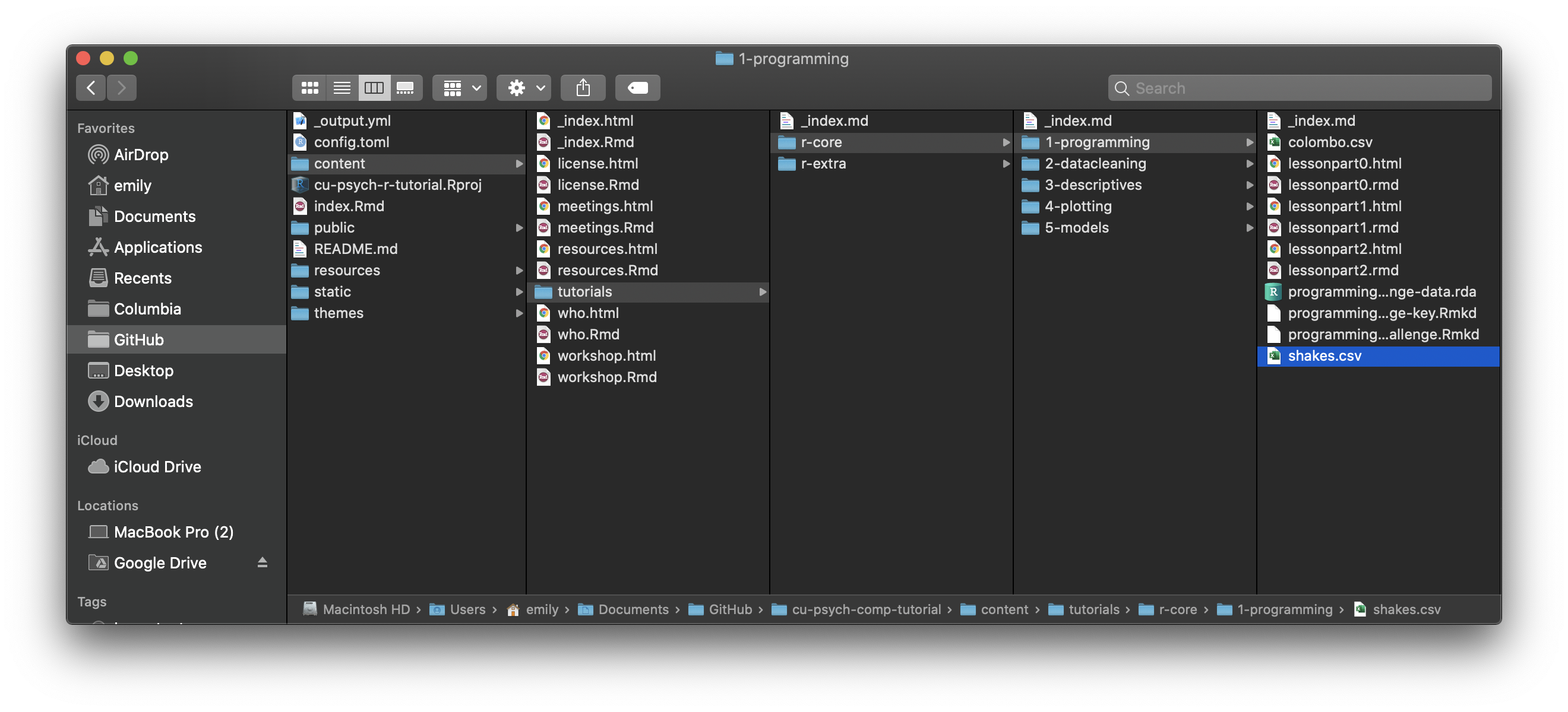
To generate a file path using here(), list the names of each subfolder in quotes, followed by the file name in quotes. Please note that these subfolder names should be listed from highest in the folder structure to lowest (ending with the subfolder where the data file is located).
## [1] "/Users/emily/Documents/GitHub/cu-psych-comp-tutorial/content/tutorials/r-core/1-programming/shakes.csv"Reading the data into R
Then, to examine this file in R, place the file path inside the parentheses in the read_csv() function. You could do this by copying and pasting the full file path outputted by the here() function, but it is simpler to “nest” the here() function inside read_csv().
## # A tibble: 37 x 3
##    title                     genre   n.words
##    <chr>                     <chr>     <dbl>
##  1 All's Well That Ends Well Comedy    23009
##  2 Antony and Cleopatra      Tragedy   24905
##  3 As You Like It            Comedy    21690
##  4 Comedy of Errors          Comedy    14701
##  5 Coriolanus                Tragedy   27589
##  6 Cymbeline                 Tragedy   27565
##  7 Hamlet                    Tragedy   30557
##  8 Henry IV, Part I          History   24579
##  9 Henry IV, Part II         History   25689
## 10 Henry V                   History   26119
## # … with 27 more rows
After running the line above, you will see a preview of the file in R. Sometimes this kind of quick preview is helpful! However, in order to do more with the data, you will want to save a copy of the file as an object in your R environment. (You can tell that the file has not yet been loaded into your environment by taking a look at the Environment tab in the upper right section of your RStudio window. Unless you were working in R before this workshop began, you will see a message noting that it is empty!)
Loading the file as an R object
To load the file into your R environment, give it a name (e.g., shakes) and use the <- (the assignment operator) to save the data contained in the CSV into an R object with that name.
Once you have done so, you will see this object listed in the Environment tab in the upper right section of your RStudio window.