Data Cleaning
Created by: Ellen Tedeschi
core
R
Goals of This Lesson
Students will learn:
- How to open various data types in R
- How to check for missing or problematic data and address issues.
- How to filter, rearrange and shape data in preparation for analysis.
Links to Files and Video Recording
The files for all tutorials can be downloaded from the Columbia Psychology Scientific Computing GitHub page using these instructions. This particular file is located here: /content/tutorials/r-core/2-datacleaning/index.rmd.
For a video recording of this tutorial from the Fall 2020 workshop, please visit the Workshop Recording: Session 2 page.
Install Packages
tidyverse is one package with many tools. Although you first encountered it in the Programming lessons, we will introduce this package further in this lesson, and will continue using tidyverse in the modules to come.
Getting Your Data into R
Entering data directly
In some cases, you may want to enter data directly into R. This is easy with a small number of cases.
# Direct Data Entry
dataframe <- tibble(name = c("Monica", "Michelle", "Paul", "Ellen"),
                    score = c(20, 16, 35, 19),
                    year = c(2, 5, 2, 1))
However, it’s easy to introduce errors this way, and with a lot of data it would get tedious.
Reading data into R
Most of the time, you’ll be reading data from an external file (e.g., .txt or .csv), or opening up an existing dataset in R. Once you find the location of your files, what you do next will depend on the file format.
What’s your working directory and where is the file you want?
Your working directory is the directory (and subdirectories) where the files you’re working with are stored. Whenever possible, you should open the files you run in R from a .Rproj link; by doing so, the folder in which that file was located will automatically be your working directory.
You can check your working directory using the here() function.
## [1] "/Users/mthieu/Repos/cu-psych-comp-tutorial"You can access a list of the files within your working directory using the list.files() function…
##  [1] "_output.yml"                  "blogdown"
##  [3] "config.toml"                  "content"
##  [5] "cu-psych-comp-tutorial.Rproj" "index.Rmd"
##  [7] "layouts"                      "public"
##  [9] "README.md"                    "renv"
## [11] "renv.lock"                    "resources"
## [13] "static"                       "themes"
…as well as in the “Files” tab in the module at the bottom right corner of your RStudio window.
What kind of file do you have?
## To load .csv files
mydata <- read_csv(here("content", "tutorials", "r-core", "2-dataCleaning", "Study1.csv"))
##
## ── Column specification ────────────────────────────────────────────────────────
## cols(
## ID = col_double(),
## Age = col_double(),
## Sex = col_character(),
## Condition = col_double(),
## Personality = col_double(),
## T1 = col_double(),
## T2 = col_double(),
## T3 = col_double(),
## T4 = col_double()
## )# Other options include:
# read_tsv, for tab-delimited files
# read_delim, for when you have a separator that's not standard
## To load data that's already in an R format
load(here("content", "tutorials", "r-core", "2-dataCleaning", "Study1.rda"))
## To load data from Excel (.xlsx, .xls):
# install.packages("readxl")
# library(readxl)
# read_excel(<Path to file>)
## To load data from many other programs (e.g., SPSS, SAS, Stata, and more):
# install.packages("foreign")
# library(foreign)
# read.spss(<Path to file>)
# read.dta(<Path to file>)Remember, all of these commands can have arguments that will help R make sense of your data. To find out what arguments are possible, put a question mark in front of the name of the function (e.g. ?read.table). For options not listed here, Google “
Inspecting Your Data
Now you have data, it’s time to get some results! But wait! Are you sure this data is ok? Performing some basic steps to inspect your data now can save you lots of headaches later, and R makes it really easy.
Start by checking that you have the expected number of rows and columns in your data frame. You can do this by looking at the Environment window, or by asking R.
How is your data frame structured?
## [1] 9## [1] "ID" "Age" "Sex" "Condition" "Personality"
## [6] "T1" "T2" "T3" "T4"## # A tibble: 50 x 9
## ID Age Sex Condition Personality T1 T2 T3 T4
## <dbl> <dbl> <chr> <dbl> <dbl> <dbl> <dbl> <dbl> <dbl>
## 1 1 21 Female 0 67 5 2 3 1
## 2 2 22 Female 1 63 4 1 5 2
## 3 3 24 Male 1 58 6 2 6 2
## 4 4 22 Female 1 51 2 3 6 5
## 5 5 19 Female 0 49 7 6 5 2
## 6 6 25 Female 1 45 6 3 6 5
## 7 7 24 Female 1 68 7 1 4 6
## 8 8 19 Male 1 58 4 7 3 4
## 9 9 21 Male 1 56 3 4 7 2
## 10 10 20 Female 0 74 6 1 6 2
## # … with 40 more rowsBrief intro to tidyverse
tidyverse is not one package; instead, it’s multiple packages grouped together. They’re all made by the same developers, so the functions play nicely together. If you’ve worked in R before, there are some packages that you’re probably familiar with, like ggplot2 and dplyr, as well as others that are more obscure. These are all very useful packages, but they do have some tidyverse-specific syntax that we’ll be using. (Note: The following paragraphs are taken almost verbatim from our standalone tidyverse tutorial).
Enter the pipe %>%! The pipe does one simple, but key, thing: takes the object on the left-hand side and feeds it into the first argument of the function on the right-hand side. This means that:
a %>% foo()is equivalent tofoo(a). Fine and good.a %>% foo() %>% bar(arg = TRUE)is equivalent tobar(foo(a), arg = TRUE). Now, nested function calls read left-to-right!- Most common use case:
df_new <- df_old %>% foo() %>% bar(arg = TRUE) %>% baz()is equivalent todf_new <- baz(bar(foo(df_old), arg = TRUE)). Now, you can chain a series of preprocessing commands to operate on a dataframe all at once, and easily read those commands as typed in your script. No more accidentally not running some key preprocessing command that causes later code to break!
Note that #pipelife requires functions to:
- take as their first argument the object to be operated upon
- return the same object (or an analog of said), but now operated upon
Essentially all functions from the tidyverse are pipe-safe (including the mutate() and summarize() functions covered in the Programming, Part 1 tutorial and the filter() function covered in the Programming, Part 2 tutorial), but bear this in mind when trying to incorporate functions from base R or other packages into your tidy new world.
Renaming a variable
We’ll demonstrate the %>% command for our first cleaning step. Look back at your mydata data frame. What is that fifth variable? What does that even mean? Luckily, this is your study and you know that it’s a personality questionnaire measuring neuroticism. Let’s fix that using recode() from the dplyr package.
# Simple command with no pipe, commented out so we don't run both.
# mydata <- rename(mydata, Neuroticism=Personality) ## NewVariableName = OldVariableName

# Simple command with pipe
mydata <- mydata %>%
  rename(Neuroticism=Personality)

mydata
## # A tibble: 50 x 9
## ID Age Sex Condition Neuroticism T1 T2 T3 T4
## <dbl> <dbl> <chr> <dbl> <dbl> <dbl> <dbl> <dbl> <dbl>
## 1 1 21 Female 0 67 5 2 3 1
## 2 2 22 Female 1 63 4 1 5 2
## 3 3 24 Male 1 58 6 2 6 2
## 4 4 22 Female 1 51 2 3 6 5
## 5 5 19 Female 0 49 7 6 5 2
## 6 6 25 Female 1 45 6 3 6 5
## 7 7 24 Female 1 68 7 1 4 6
## 8 8 19 Male 1 58 4 7 3 4
## 9 9 21 Male 1 56 3 4 7 2
## 10 10 20 Female 0 74 6 1 6 2
## # … with 40 more rowsIt might seem like the first version is simpler, but it won’t be once you start stacking functions together. For example, let’s rearrange our variables (using select()) while also renaming the variables called T1, T2, T3, and T4. Note that we keep adding %>% between each set of functions.
mydata <- mydata %>%
  rename(Day1 = T1, Day2 = T2, Day3 = T3, Day4 = T4) %>%
  select(ID, Condition, Age, everything())
mydata
## # A tibble: 50 x 9
## ID Condition Age Sex Neuroticism Day1 Day2 Day3 Day4
## <dbl> <dbl> <dbl> <chr> <dbl> <dbl> <dbl> <dbl> <dbl>
## 1 1 0 21 Female 67 5 2 3 1
## 2 2 1 22 Female 63 4 1 5 2
## 3 3 1 24 Male 58 6 2 6 2
## 4 4 1 22 Female 51 2 3 6 5
## 5 5 0 19 Female 49 7 6 5 2
## 6 6 1 25 Female 45 6 3 6 5
## 7 7 1 24 Female 68 7 1 4 6
## 8 8 1 19 Male 58 4 7 3 4
## 9 9 1 21 Male 56 3 4 7 2
## 10 10 0 20 Female 74 6 1 6 2
## # … with 40 more rowsChecking for missing data
One problem you may have is missing data. Sometimes this is something you already know about, but you should check your data frame anyway to make sure nothing was missed in a data entry error. For small datasets, you can do this visually, but for larger ones you can ask R.
## # A tibble: 1 x 9
##      ID Condition   Age Sex    Neuroticism  Day1  Day2  Day3  Day4
##   <dbl>     <dbl> <dbl> <chr>        <dbl> <dbl> <dbl> <dbl> <dbl>
## 1    39         1    NA Female          53     1     3     1     3
In this case, the missing value is the Age value in row 39. You know you have this info somewhere on a paper form, so you go dig it up and want to replace it.
Checking for correct values
To look at some of the other variables, let’s use the table() function. This works well for factors or variables with only a few different values. Our condition and sex variables are good here.
##
##  0  1
## 22 28##
## Female Femle Male
## 21 3 26When we look at the table for the Sex variable, we see another data entry problem. We have a third category that should really be another case of “Female”. Here we are going to use the function recode from the dplyr package.
# Replace bad category label
mydata <- mydata %>%
  mutate(Sex = dplyr::recode(Sex, Femle = "Female"))

table(mydata$Sex)
##
## Female Male
## 24 26##
## 18 19 20 21 22 23 24 25 30
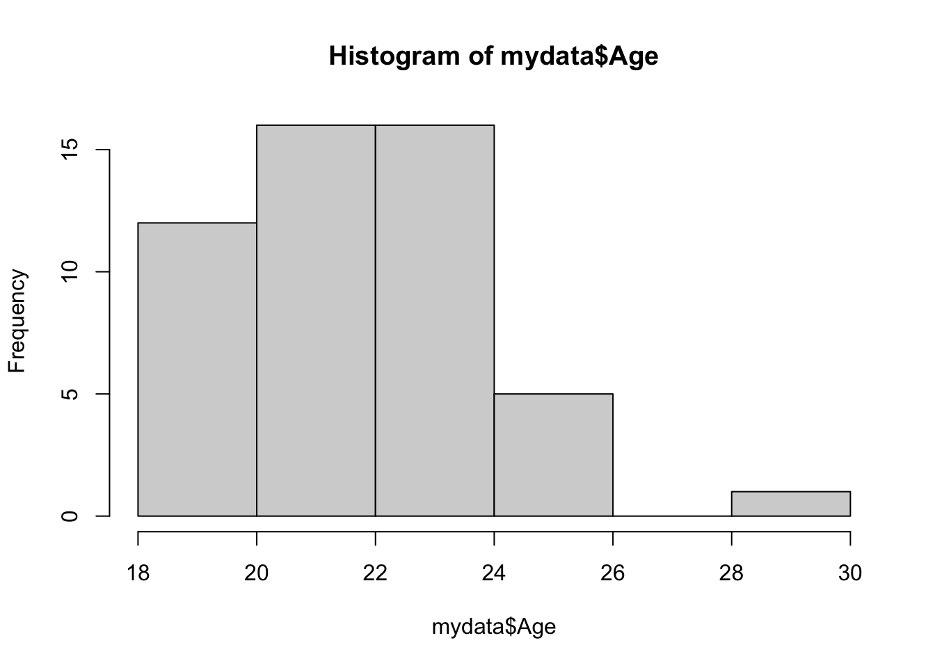
## 3 5 4 10 6 8 8 5 1Now let’s look at the continuous variables. You can also look at these with the table() function, but sometimes it’s easier to visualize. The hist() function, which creates histograms, is useful here.
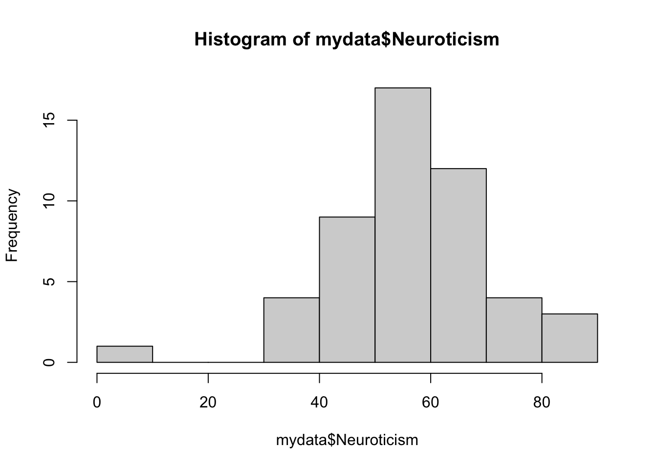
Looks like we have a potential outlier on the neuroticism score. This could be an entry error, but it could also be a real value that just happens to be really low. This is why data inspection is so important for later analysis – now that you know that value is there, it’s up to you to decide how to deal with it.
Filtering data
Let’s say we have decided a prori to exclude outliers 3SD above or below the mean. We will use the filter() function in tidyverse to clean the dataset.
# mark upper and lower boundaries of data
# anything above upper or below lower will be excluded as outlier.
upper <- mean(mydata$Neuroticism) + 3*sd(mydata$Neuroticism)
lower <- mean(mydata$Neuroticism)- 3*sd(mydata$Neuroticism)

mydata <- mydata %>%
  # only keep values within this range!
  filter( Neuroticism > lower & Neuroticism < upper)

# check that we excluded 1 outlier.
nrow(mydata)
## [1] 49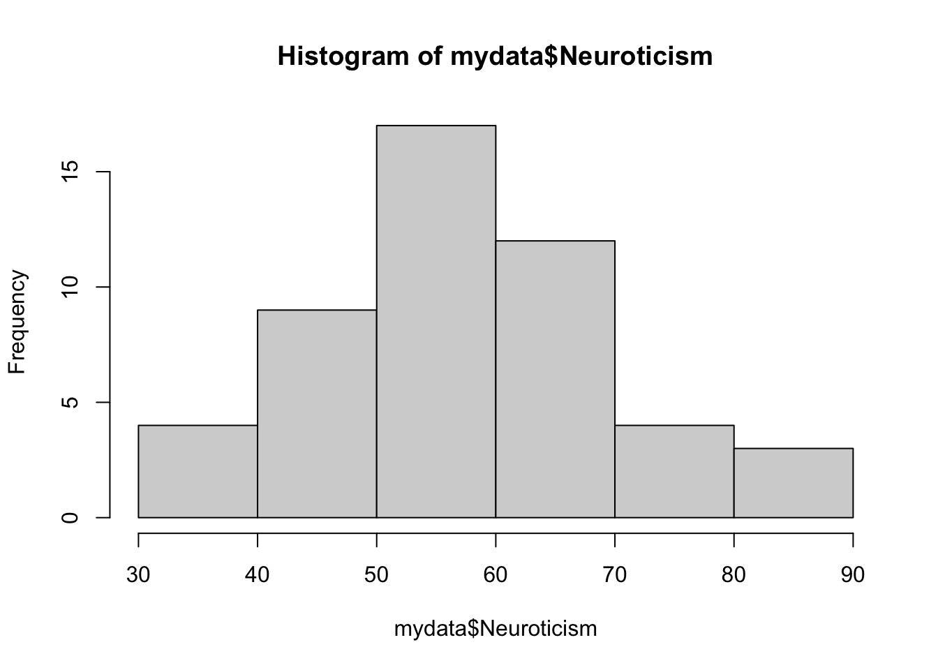
Getting Ready for Analysis
Now that we’ve gone through and cleaned up the problems, you can think ahead to how you’ll want to use this data.
Recoding variables
Sometimes we want to treat categorical variables as factors, but sometimes we want to pretend they’re numeric (as in a regression, when binary variables can be coded as 0 and 1). Right now, Condition is coded as a binary numeric variable, but that’s not very informative, and you might prefer that the values be descriptive. Here, the function recode() from the dplyr package is really useful again, but we’re going to use a different version that will also turn the variable from numeric into factor data. We’ll also create a second variable instead of overwriting Condition.
# Transform into factor with labels using mutate() and recode_factor()
mydata <- mydata %>%
  mutate(ConditionF = recode_factor(Condition, '0'='Control', '1'='Treatment'))

# Check that your variable is now recoded as you'd like!
summary(mydata$ConditionF)
## Control Treatment
## 22 27Calculating new variables
You may also want to recalculate or rescale some variables. For example, we can turn Neuroticism into a z-score, or calculate an average response across the four time points. Here we are using mutate(), a dplyr function used for adding new variables to a data frame. Mutate is nice because it makes use of other functions, such as scale() to make z-scores or rowMeans() to calculate means.
# calculate Z scores using mutate()  and scale()
mydata <- mydata %>%
  mutate(NeuroticismZ = scale(Neuroticism, center = TRUE, scale = TRUE),
         # Scale creates a matrix with width 1,
         # sometimes this messes things up so we'll convert it to vector
         NeuroticismZ = c(NeuroticismZ))

hist(mydata$NeuroticismZ)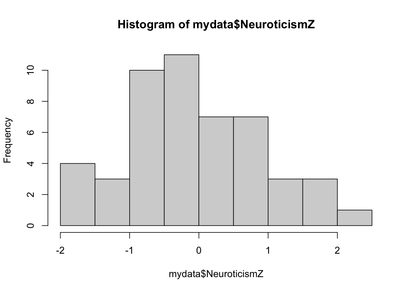
Combining data from multiple sources
Sometimes, data might be spread across multiple spreadsheets, and you’ll want to combine those for your analysis. For example, maybe this study had a follow-up survey on Day 30. Scores from that survey were entered into another spreadsheet, which only has the subject ID and that score. We want to include that score into our data.
Although there are many different functions you can use to combine data frames, here I’m using the function inner_join(), which is also part of the tidyverse.
# First load the new data
mydata2 <- read_csv(here("content", "tutorials", "r-core", "2-dataCleaning", "Study1_Followup.csv"))
##
## ── Column specification ────────────────────────────────────────────────────────
## cols(
## ID = col_double(),
## Day30 = col_double()
## )# Merge the two data frames. To make sure the rows match up, we use the 'by' argument to specify that IDs should match. That way even if the data is in a different order you will get scores matched togther correctly.
mydata <- inner_join(mydata, mydata2, by = "ID")
# Note that mydata has one less row than mydata2 because we removed that outlier. By default, inner_join will use only cases of the 'by' variable that exist in both dataframes, so it drops that one row from mydata2 when merging. You can use other _join functions if you want to keep all observations from one or both frames, even if it means blank cells.Reshaping data
Finally, you may want to change the layout of your data. Right now, our data frame is in “wide” format, which means that each row is a subject, and each observation gets its own column. For some analyses, you’ll need to use “long” format, where each row is an observation, and columns specify things like time and ID to differentiate the observations. There are lots of packages that can handle data reshaping, but I’ll show the pivot_longer() and pivot_wider() functions from tidyr.
# names_to is the name for the new column that will identify which observation it is
# values_to is the name for the new column that will have the actual values in it.
# In theory, you can name these whatever you want,
# but to keep everyone on the same page, name the key "Time" and the value "Score".

mydata_Long <- pivot_longer(mydata, cols = starts_with("Day"),
                            names_to="Time", values_to="Score")


# pivot_wider() lets you go back the other direction.
# This should be identical to the original mydata.

mydata_Wide <- pivot_wider(mydata_Long,
                           id_cols = c(ID, Age, Sex, Condition, Neuroticism),
                           names_from = Time, values_from = Score)
Saving Your Work
Once you’ve created a data cleaning script like this one, you’ll have a record of all the edits you’ve made on the raw data, and you can recreate your cleaned data just by running the script again. However, it’s often easier to save your cleaned data as its own file (never overwrite the raw data), so when you come back to do analysis you don’t have to bother with all the cleaning steps.
You can always save data frames as a .csv for easy sharing and viewing outside of R.
# Write data to a .csv
write_csv(mydata, path = here("content", "tutorials", "r-core", "2-dataCleaning", "Study1_Clean.csv"))
However, you can also save in an R format that lets you save multiple variables/objects in the same file. For example, you might want to have a long and wide format, or one dataframe with all the data and one with just subject information. Saving as a .rda file allows you to save multiple objects at once for easy loading into R. You can also save the outputs of statistical models in these, along with their data.
Future Directions
Congratulations! You’ve now cleaned some data in R and you’re ready to start working with your data. This tutorial only went over some basic cleaning steps. As you work with your own data, you may find yourself needing other tools.
Next: Data Manipulation (Grouping, categorizing, and descriptive statistics)