Intro to RMarkdown
Created by: Emily Nakkawita
extra
R
Links to Files
The files for all tutorials can be downloaded from the Columbia Psychology Scientific Computing GitHub page using these instructions. This particular file is located here: /content/tutorials/r-extra/rmarkdown/intro-to-rmarkdown.rmd.
Getting started
To work with R Markdown, if necessary:
- Install R
- Install the latest version of RStudio
- Install the latest version of the
knitrpackage:install.packages("knitr")
If you’re looking for a quick reference to R Markdown formatting, I strongly suggest you check out this helpful cheat sheet!
R Markdown formatting
In R Markdown, you can type normally as you would in a simple text document. This text can be interspersed with R code in what are called chunks. The ability to combine text and R code means that you can develop papers, manuscripts, presentations, and web pages (and more!) within a single document.
In order to see the code used to generate the formatting you’ll see in the output document, we recommend you open to R Markdown (.Rmd) file as well as the final outputted PDF.
Text formatting
You can italicize text by placing it inside of a single set of asterisks (*) or underscores (_).
You can bold text by placing it inside of a double set of asterisks (**) or underscores(__).
Headers are created by starting a line with a specific number of pound or hash signs (#) that corresponds with the level of your header. For example:
First-level header
Second-level header
Third-level header
Fourth-level header
Fifth-level header
Lists
An unordered list (with bullet points) can be created by typing an asterisk and space (*) at the beginning of each line. Second-level sub-bullets can be created by typing tab twice and then typing a hyphen and a space (-) at the beginning of each line. (I think on some computers sub-bullets may work if you type tab once, but it doesn’t on my Mac!)
- Bullet 1
- Sub-bullet 1
- Sub-bullet 2
- Bullet 2
- Bullet 3
Please note: You’ll need to leave a blank line in your .Rmd file before the first bullet or it won’t output properly.
An ordered list (with numbers) can be created by typing a number, period, and space (e.g., 1.) at the beginning of each line. Second-level sub-bullets can be created by typing tab twice and then typing “i”, a right parenthesis, and a space (i)) at the beginning of each line. (With each new line, you’ll increase your “i”s as this is written in lowercase Roman numerals.)
- Number 1
- Sub-bullet 1
- Sub-bullet 2
- Number 2
- Number 3
Equations
You can add equations to your R Markdown file by including them either between single dollar signs (for inline equations within your text) or double dollar signs (for a separate equation section below your text–often used to highlight formulas in papers). This is based on something called LaTeX notation.
Here is an example of an inline equation: \(y_i = \alpha + \beta x_i + e_i\).
Here is a displayed formula:
\[\frac{1}{1+\exp(-x)}\]
Hyperlinks
You can add a hyperlink by typing the text you’d like to link in brackets followed by the URL in parentheses with no space between them. Here is an example.
Images
The code to include an image is similar to that for a hyperlink. You’ll type an exlamation point, followed by the image caption in brackets, followed by the image location (either a URL or a path to the image’s location on your computer) with no spaces between them. The image here is a bit large, so you’ll see that RMarkdown pushed it to the next page in the knitted PDF document.

Butler Library
Quotes
Quotes can be included by typing a greater-than sign and space at the beginning of each line (>).
To be, or not to be, that is the question: Whether ’tis nobler in the mind to suffer The slings and arrows of outrageous fortune…
Tables
Basic tables can be included using the following notation:
| A | B | C |
|---|---|---|
| 1 | Male | Blue |
| 2 | Female | Pink |
You can also include tables within code chunks, which will be illustrated in the next section.
Code
Code chunks
Most of the time, you’ll use code chunks within R Markdown to run your code. Here is an example code chunk. (I’ve also created some dummy data here we’ll use to demonstrate functions in subsequent code chunks.)
```r
x <- c(1, 2, 4, 4, 5, 5, 5, 7, 9, 9)
y <- 1:10
df <- data.frame(x, y)
x
```

```
##  [1] 1 2 4 4 5 5 5 7 9 9
```
To insert an R code chunk, you can type it manually or use the shortcut key (Ctrl-Alt-I on PC; Cmd-Option-I on Mac). This will produce the following code chunk:
Inline code
Inline code can be included by placing your code in and starting it with r and a space. (If you’re viewing this in the PDF, see the .Rmd file for the code.) Inline code can be a really helpful way to pull out a datapoint and include it in your text. For example, here is the second value in our vector x : 2.
Tables (from code chunks)
You can create a table of a dataframe by placing the dataframe name within the kable() function.
| x | y |
|---|---|
| 1 | 1 |
| 2 | 2 |
| 4 | 3 |
| 4 | 4 |
| 5 | 5 |
| 5 | 6 |
| 5 | 7 |
| 7 | 8 |
| 9 | 9 |
| 9 | 10 |
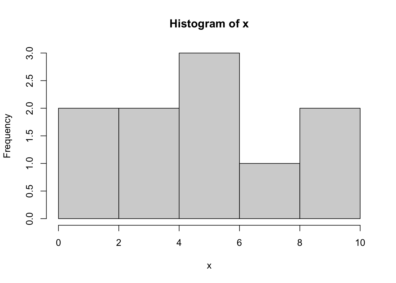
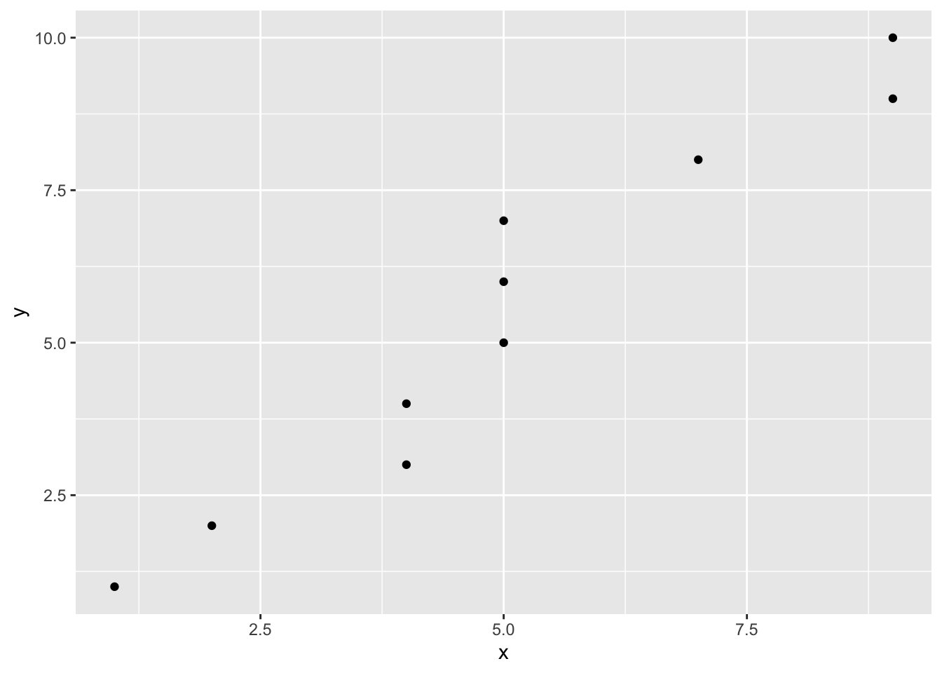
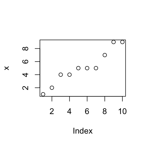
Plots
Images generated by knitr are saved in a figures folder.
Code chunk options
There are a wide range of code chunk options, which you can find listed in this helpful cheat sheet. We highlight some of the most common here.
eval: Evaluate the code in the chunk (or not)
You can tell R not to evaluate (i.e., run) the code in a particular chunk by inserting eval = FALSE at the beginning of your code chunk.
```r
# We included the eval = FALSE option at the beginning of this chunk
y <- 0
```


```r
# We can check here and see that the change in the previous chunk was not made to y
# because the code wasn't evaluated.
y
```

```
##  [1]  1  2  3  4  5  6  7  8  9 10
```cache: Save a copy of your analysis (or not)
You can cache the results of your analyses if the analyses take a long time to run. If you insert cache = TRUE at the beginning of your code chunk, the analysis will run in full the first time you knit the file; in future knits, the code will not be re-run.
If you want to re-run cached code chunks, just delete the contents of the cache folder.
```r
for (i in 1:5000) {
    lm((i+1)~i)
}
```echo: Show vs. hide command input
The echo = FALSE code hides the code within the code chunk within your output file but still runs the code. results = 'asis' here formats the output to match your document format (i.e., not to look like code output in the Courier font).
Here are some points within our y vector
- The value of y[1] is 1
- The value of y[2] is 2
- The value of y[3] is 3
R Markdown file types
There are a wide range of files you can create using R Markdown, but the options you’ll probably use most commonly are a PDF, Word document, and HTML file. To change the output file type, change the output: line in your .Rmd header based on your desired file type:
- PDF:
pdf_document - Word:
word_document - HTML:
html_document