Tidy Walkthrough, Part 2

Created by: Monica Thieu extra R

Goals for this vignette

Hello (again)! This is a continuation of our tour through base tidyverse (see Part 1 here). Our goals are the same as before:

Demonstrate (what I think are) key first-level features of the tidyverse
Illustrate psychology use cases for tidyverse functions
Hopefully convince you to join the cult of tidy

This time, we’ll be moving ahead to some more complex use cases utilizing some more advanced programming tactics. I hope to show you how the tidyverse makes these things a little smoother!

Again, please remember that for more exhaustive documentation you can visit the online reference pages for your package of interest, and for more in-depth self-teaching, please refer to the R for Data Science online textbook by Garrett Grolemund and Hadley Wickham.

Links to Files

The files for all tutorials can be downloaded from the Columbia Psychology Scientific Computing GitHub page using these instructions. This particular file is located here: /content/tutorials/r-extra/tidyverse-guide/tidyguide-2.rmd.

Quick cheat-list of key functions from various pkgs

These are not the only functions in these packages that you may find useful! These are simply the functions from these packages that will be featured in this vignette.

dplyr
- the *_join() family of functions to join dfs row-wise by key columns
tidyr
- nest() and unnest() to wrap/unwrap a long-form df to/from a nested df with list-columns of observation-level data
purrr
- the map() family of vectorizing helper functions
broom
- tidy() to extract coefficients/SEs from models as a df

Initializing fake data

We’ll use a simulated dataset for this vignette, so you don’t need to worry about any dependencies involving datasets you don’t have access to while you’re following along.

If you have tidyverse loaded, all this code should run if you try to run it in your R console.

If you’re coming from part 1 of our tidyverse tour, this is the exact same simulated raw data as before. As a reminder, this is a simulated recognition memory task, where for a series of objects that were either seen or not seen in a previous learning phase, fake subjects must respond “old” if they think they saw the object before, and “new” if they think they did not.

# 20 fake subjects, 50 fake trials per subject

# Will simulate the person-level variables FIRST,
# then expand to simulate the trial-level variables
raw <- tibble(id = 1L:20L,
              age = sample(18L:35L, size = 20, replace = TRUE),
              # assuming binary gender for the purposes of this simulation
              gender = sample(c("male", "female"), size = 20, replace = TRUE)) %>%
  # simulating some "questionnaire" scores; person-level
  mutate(q_1 = rnorm(n = n(), mean = 30, sd = 10),
              q_2 = rnorm(n = n(), mean = 30, sd = 10),
              q_3 = rnorm(n = n(), mean = 30, sd = 10)) %>%
  # slice() subsets rows by position; you can use it to repeat rows by repeating position indices
  slice(rep(1:n(), each = 50)) %>%
  # We'll get to this in a bit--this causes every "group"
  # aka every set of rows with the same value for "id", to behave as an independent df
  group_by(id) %>%
  # I just want to have a column for "trial order", I like those in my task data
  mutate(trial_num = 1:n(),
         # Each subject sees half OLD and half NEW trials in this recognition memory task
         is_old = rep(0L:1L, times = n()/2),
         # I'm shuffling the order of "old" and "new" trials in my fake memory task
         is_old = sample(is_old),
         # This will generate binary "old"/"new" responses corresponding roughly to a d' of 1
         # yep, everyone has the same d' today
         response = if_else(is_old == 1,
                            rbinom(n = n(), size = 1, prob = 0.7),
                            rbinom(n = n(), size = 1, prob = 0.3)),
         rt = rnorm(n = n(), mean = 3, sd = 1.5)) %>%
  ungroup()

Joining dfs

Under construction!

Nested dfs

Nearly all of the tidyverse features we’ll be working through in this vignette rely on two key features of R to make their magic happen: list-columns and flexible vectorizing functions. These are features that you may very well encounter explicitly in casual R usage, so we’ll take a bit of time to familiarize ourselves with these concepts before we jump all the way in.

A brief (re)view of lists

Your usual vector, be it character, numeric, or logical, is an atomic vector–this means that every element in the vector is required to be the same data type. A list is also a vector, but it’s not bound to be atomic. The different elements of a list do not have to be the same data type. They don’t even all have to be length 1!

If you’re familiar with data types in Matlab, a list is very similar to a Matlab struct array. Both are objects that contain multiple elements that aren’t bound to be the same type, or length 1.

While you might initialize an atomic vector using c(), you have to use list() to initialize list vectors.

mylist <- list(1,
               "one",
               c(1, 11, 111))

mylist

## [[1]]
## [1] 1
## 
## [[2]]
## [1] "one"
## 
## [[3]]
## [1]   1  11 111

Notice how R shows you the bracket indexing of the list elements above. There are two ways to bracket index list vectors, with single brackets [] and double brackets [[]].

Single-bracket indexing a list vector always returns another list object.

mylist[1]

## [[1]]
## [1] 1

mylist[2:3]

## [[1]]
## [1] "one"
## 
## [[2]]
## [1]   1  11 111

See above that when you print single-bracket indexed lists to console, you still get console output that shows you each list element under double-bracketed indices.

typeof(mylist[2:3])

## [1] "list"

More explicitly, you can see that single-bracket indexing a list will return an object of list type.

Meanwhile, double-bracket indexing a list vector returns the object stored inside that list field.

mylist[[2]]

## [1] "one"

mylist[[3]]

## [1]   1  11 111

Above, you actually get the object stored inside the list at the relevant element. This is probably what you’re expecting when you index a list–to unlist or “unwrap” the element on the inside you wish to access.

typeof(mylist[[3]])

## [1] "double"

Just making sure that it is in fact the type of the element stored inside, and no longer list type.

Notice that you can return an indexed list object of any length when you single-bracket index, but double-bracket indexing to extract individual list elements only lets you access one at a time!

A feature of lists that can be very useful is that list elements can have names. You can create a named list object by naming list elements when you specify them:

mylist <- list(first = 1,
               second = "one",
               third = c(1, 11, 111))

mylist

## $first
## [1] 1
## 
## $second
## [1] "one"
## 
## $third
## [1]   1  11 111

When a list has named elements, printing the list to console will show you the names of the elements. Handy!

The best thing about named list elements is that you can use those names to access list elements!

mylist["first"]

## $first
## [1] 1

mylist[c("second", "third")]

## $second
## [1] "one"
## 
## $third
## [1]   1  11 111

mylist[["first"]]

## [1] 1

Again, single-bracket indexing continues to return a list (this time, a named list containing the elements you indexed), and allows you to index multiple elements at once by feeding in a character vector of names. Double-bracket indexing, meanwhile, unwraps the element you’re indexing.

You can also index named lists with the dollar sign $ operator! Seem familiar?

mylist$third

## [1]   1  11 111

This is the same way you index df columns! In fact, somewhere deep down, a dataframe/tibble is a very special list, where each list element is required to be a vector of the same length. Isn’t that cool?

That’s the basics you need to know about lists, summarized here just in case:

it’s a vector, basically
it contains different elements that are not bound to be the same type, and can be vectors themselves
Single-bracket indexing returns a list, while double-bracket indexing unwraps the element
elements can have names, which allows indexing by name using brackets or $

Lists as df columns

A df is composed of columns, each of which is a vector of identical length. But nobody ever said the columns of a df all have to be atomic vectors! A df column can be a list vector, where each element of said list-column can contain objects of different data types and lengths.

This becomes a little easier to wrap your head around if we explicitly look at a df with list-columns in it. Below, we’ll take a look at the starwars df, which is a toy dataset about Star Wars characters that comes standard with dplyr.

starwars

## # A tibble: 87 x 14
##    name  height  mass hair_color skin_color eye_color birth_year sex   gender
##    <chr>  <int> <dbl> <chr>      <chr>      <chr>          <dbl> <chr> <chr> 
##  1 Luke…    172    77 blond      fair       blue            19   male  mascu…
##  2 C-3PO    167    75 <NA>       gold       yellow         112   none  mascu…
##  3 R2-D2     96    32 <NA>       white, bl… red             33   none  mascu…
##  4 Dart…    202   136 none       white      yellow          41.9 male  mascu…
##  5 Leia…    150    49 brown      light      brown           19   fema… femin…
##  6 Owen…    178   120 brown, gr… light      blue            52   male  mascu…
##  7 Beru…    165    75 brown      light      blue            47   fema… femin…
##  8 R5-D4     97    32 <NA>       white, red red             NA   none  mascu…
##  9 Bigg…    183    84 black      light      brown           24   male  mascu…
## 10 Obi-…    182    77 auburn, w… fair       blue-gray       57   male  mascu…
## # … with 77 more rows, and 5 more variables: homeworld <chr>, species <chr>,
## #   films <list>, vehicles <list>, starships <list>

In this df, each row is a “subject” (a character from the movies). Currently, this data is “tidy”: each row is a unique observation (subject in this case), and each column is a distinct variable giving information about that observation.

Because this object is a tibble (makes sense since it comes with dplyr), we can inspect the nice print output to see the types of the different columns. We can see that the first few columns are atomic vectors, either numeric like height and mass or character like homeworld. But check out the last three columns…

starwars %>%
  select(name, films, vehicles, starships)

## # A tibble: 87 x 4
##    name               films     vehicles  starships
##    <chr>              <list>    <list>    <list>   
##  1 Luke Skywalker     <chr [5]> <chr [2]> <chr [2]>
##  2 C-3PO              <chr [6]> <chr [0]> <chr [0]>
##  3 R2-D2              <chr [7]> <chr [0]> <chr [0]>
##  4 Darth Vader        <chr [4]> <chr [0]> <chr [1]>
##  5 Leia Organa        <chr [5]> <chr [1]> <chr [0]>
##  6 Owen Lars          <chr [3]> <chr [0]> <chr [0]>
##  7 Beru Whitesun lars <chr [3]> <chr [0]> <chr [0]>
##  8 R5-D4              <chr [1]> <chr [0]> <chr [0]>
##  9 Biggs Darklighter  <chr [1]> <chr [0]> <chr [1]>
## 10 Obi-Wan Kenobi     <chr [6]> <chr [1]> <chr [5]>
## # … with 77 more rows

The last three columns are list type! This makes sense based on the content we might expect to be contained within each column. For example, if each row is one character, but one character appears in multiple movies, you might expect that character’s value in the films column to contain a vector with one element for each movie that character was in. In this way, a list-column allows you to store multiple observations per subject wrapped up in such a way that the main df still has one row per subject, but you retain the observation-level data because you haven’t actually collapsed across any variables.

(You’re probably familiar with fully long-form data, where each observation has its own row, and then grouping variables like subject are repeated for all observations that belong to the same subject. We will learn about the relationship between dfs containing list-columns and fully long-form dfs later!)

Now, for list-columns, instead of actually printing the content of the vector, tibble output gives us a blurb about the object contained inside of each list element. To inspect the contents of a list-column, we have to index into the list-column using one of the techniques we reviewed above.

We can index by position, which corresponds to row numbers, using single-bracket indexing to return another, shorter list:

# These should be Luke's starships that he piloted at some point in the series
# since we saw earlier that he's the first row of the df
starwars$starships[1]

## [[1]]
## [1] "X-wing"           "Imperial shuttle"

Or double-bracket indexing, which allows us to actually access the object contained within:

starwars$starships[[1]]

## [1] "X-wing"           "Imperial shuttle"

We can also use logical indexing to access list-column elements based on values in other columns.

# This is good when you don't necessarily know the row number of what you're looking for
starwars$starships[starwars$name == "Han Solo"]

## [[1]]
## [1] "Millennium Falcon" "Imperial shuttle"

Note that logical indexing only works with single-bracket indexing. If you want to unwrap the object contained within, you have to index twice like below:

starwars$starships[starwars$name == "Han Solo"][[1]]

## [1] "Millennium Falcon" "Imperial shuttle"

This works because single-bracket indexing always returns another list, and you can then double-bracket index into THAT list. It’s a lot of brackets, but it does follow a pattern!

A df with a list-column still behaves like a df, mostly

If your df contains a list-column, you can do most things with that df that you might do with a fully atomic list-free df. You can:

subset by column using select()
reshape your df using pivot_longer() and pivot_wider()

There are a couple respects in which list-columns are limited, though. Most of these involve the fact that R makes fewer assumptions about the content of lists (since elements are not bound to be the same type/length 1), and so for your own safety the tidyverse prevents you from doing some things that might yield unexpected results:

you cannot directly filter() or distinct() a df by a list-column, but you can do these things to a df containing list-columns by an atomic column
you cannot group_by() a df by a list-column, but you can group_by() atomic columns in a df containing list-columns

What about using mutate() to create/modify list-columns? You can do this, but it requires special vectorizing functions like purrr::map() that we will cover later. Stay tuned!

df-ception: df list-columns that contain other dfs

Okay, so now that you’ve seen list-columns that contain different atomic vectors, it’s time to get list-crazy! A list really can contain basically anything in each of its elements. This means that a list can contain a whole df inside of one (or more) of its list elements.

When would you want a df that contains other dfs? Well, remember that list-columns are typically useful to contain multiple observations of information that pertain to one subject/group/etc while allowing your df to take a one-row-per-subject/group structure.

You usually won’t be creating dfs with df-containing list-columns from scratch. More likely, you’ll start with a fully long df, and condense the repeated measures data by folding it into a list-column using tidyr::nest(). Let’s try it with the starwars df, by creating a df that has one row per species x homeworld, and a list-column containing a df for all of the characters of a particular species/homeworld grouping.

starwars_by_species_home <- starwars %>%
  nest(characters = -c(species, homeworld))

starwars_by_species_home

## # A tibble: 58 x 3
##    homeworld species characters       
##    <chr>     <chr>   <list>           
##  1 Tatooine  Human   <tibble [8 × 12]>
##  2 Tatooine  Droid   <tibble [2 × 12]>
##  3 Naboo     Droid   <tibble [1 × 12]>
##  4 Alderaan  Human   <tibble [3 × 12]>
##  5 Stewjon   Human   <tibble [1 × 12]>
##  6 Eriadu    Human   <tibble [1 × 12]>
##  7 Kashyyyk  Wookiee <tibble [2 × 12]>
##  8 Corellia  Human   <tibble [2 × 12]>
##  9 Rodia     Rodian  <tibble [1 × 12]>
## 10 Nal Hutta Hutt    <tibble [1 × 12]>
## # … with 48 more rows

We’ve done two things here:

We folded all the observations into a separate column called characters using nest(),
We used a negative vector to hold grouping-level variables out of that folded column

nest() is what you’ll use to create nested dfs, or dfs with columns containing other dfs. nest() takes every column that isn’t a grouping variable, and folds all of the observations in each group into their own df in the new list-column. All the data we had before is inside this new list-column. Let’s look inside one of these sub-dfs to be sure:

starwars_by_species_home$characters[[1]]

## # A tibble: 8 x 12
##   name  height  mass hair_color skin_color eye_color birth_year sex   gender
##   <chr>  <int> <dbl> <chr>      <chr>      <chr>          <dbl> <chr> <chr> 
## 1 Luke…    172    77 blond      fair       blue            19   male  mascu…
## 2 Dart…    202   136 none       white      yellow          41.9 male  mascu…
## 3 Owen…    178   120 brown, gr… light      blue            52   male  mascu…
## 4 Beru…    165    75 brown      light      blue            47   fema… femin…
## 5 Bigg…    183    84 black      light      brown           24   male  mascu…
## 6 Anak…    188    84 blond      fair       blue            41.9 male  mascu…
## 7 Shmi…    163    NA black      fair       brown           72   fema… femin…
## 8 Clie…    183    NA brown      fair       blue            82   male  mascu…
## # … with 3 more variables: films <list>, vehicles <list>, starships <list>

In our new nested df, the first row contains all Star Wars characters who are humans from Tatooine. Thus, if we look inside the df stored in the first element of the characters list-column using double-bracket indexing, we see all of the original character-level observations belonging to this group. Notice that inside this sub-df, the columns species and homeworld are absent. This is because these columns are already present in the main df, as the grouping variables.

You can nest() with as many or as few grouping variables as you’d like–anything that you can group_by() you can nest() along.

If you have a nested df that you would like to unnest, and return to fully long form, you can do that using tidyr::unnest(). As you might guess, unnest() essentially does the exact opposite of nest()– it takes list-columns and unfolds them back out to be one row per observation instead of one row per group.

starwars_by_species_home %>%
  unnest(characters)

## # A tibble: 87 x 14
##    homeworld species name  height  mass hair_color skin_color eye_color
##    <chr>     <chr>   <chr>  <int> <dbl> <chr>      <chr>      <chr>    
##  1 Tatooine  Human   Luke…    172    77 blond      fair       blue     
##  2 Tatooine  Human   Dart…    202   136 none       white      yellow   
##  3 Tatooine  Human   Owen…    178   120 brown, gr… light      blue     
##  4 Tatooine  Human   Beru…    165    75 brown      light      blue     
##  5 Tatooine  Human   Bigg…    183    84 black      light      brown    
##  6 Tatooine  Human   Anak…    188    84 blond      fair       blue     
##  7 Tatooine  Human   Shmi…    163    NA black      fair       brown    
##  8 Tatooine  Human   Clie…    183    NA brown      fair       blue     
##  9 Tatooine  Droid   C-3PO    167    75 <NA>       gold       yellow   
## 10 Tatooine  Droid   R5-D4     97    32 <NA>       white, red red      
## # … with 77 more rows, and 6 more variables: birth_year <dbl>, sex <chr>,
## #   gender <chr>, films <list>, vehicles <list>, starships <list>

There we go, this should be the same df as before! As shown above, unnest() takes the names of columns to be unnested as arguments. I like to always specify the column(s) I’d like to unnest for maximum readability, so it’s obvious to future you/other collaborators exactly what you’re nesting.

You’ll see that the rows have been re-ordered according to the previous nested grouping, so keep this in mind if you’re expecting rows to be in a particular order (you may need to re-order your df using arrange() after unnesting).

What are nested dfs useful for?

For the most part, straightforward data manipulation operations are easier to do on fully long dfs than they are on nested dfs, for reasons we’ll get to soon. You won’t need to use a nested df all the time, and that’s okay! Nested dfs are really great for allowing you to do summarizing and modeling operations alongside your observation-level data, without discarding it. We’ll be learning about this below, so don’t forget about nested dfs because they are coming back!

Vectorizing to the high heavens

Next, we’ll review vectorizing: this is a feature of R that you probably use all the time and don’t even know it! We’ll learn a little more about what vectorized functions do and how you can vectorize any function you wish.

To read more in-depth about vectorized functions in R, check out this handy blog post from Noam Ross. We won’t be getting deep into the nuts and bolts of how vectorization works in R here. We’ll just be discussing it at a high level that should orient you enough to be able to make quick use of vectorizing helper functions.

purrr::map() goes here? compare to apply family of functions in base R

Vectorizing: it’s like a for loop, but not

As you’ve likely experienced, much data processing requires writing code to perform a particular action, and then wrapping it in other code to repeat that action many times over many objects. In R, this usually means doing the same operation to every element in a vector or every row in a df column.

In most computing languages, the most sensible way to do one thing a bunch of times is to use a for loop, which (I know you know this but I’ll spell it out just to be extra) repeats the code inside the loop once for every element of a vector that’s specified at the beginning of the loop code.

To use a for loop to apply some function to every element of a df column, you might write something like:

for (i in 1:nrow(df)) {
  df$new_col[i] = my_function(df$old_col[i])
}

and that would do the trick. In this case, the vector you iterate along contains the row indices of your df, which means that on every iteration of your loop you’re calling my_function() on the next row of data until you get to the end of your df.

This is a perfectly functional way to write code! Today, I’ll argue that it’s prone to typos that might cause you big headaches. Specifically, these typos may cause your code to fail silently (ominous organ riff), or do something unintended without throwing an error. This means you wouldn’t find out that something was wrong unless you visually inspected the output, which you can’t always do after every command (I getcha). Thus, there’s a risk of inducing mistakes in the data that you don’t catch until it’s too late.

For example, once I wrote a for loop just like the above, to perform some functions on every row of a df column, but I wrote df$old_col[1] instead of df$old_col[i]. I accidentally had the same value in every element of df$new_col, because even though the for loop was iterating as usual, on every iteration of the loop it was calling the same value. I didn’t discover my typo until weeks later. No bueno!

Enter… vectorizing.

It turns out that R has built-in optimized functionality for repeating functions along every element of a vector, just waiting for you to harness!

Generally, any vectorized function takes a vector as input, does the same thing to every element of that vector, and returns a vector of the same length as output. Plenty of functions are already vectorized, and you likely already use them as such, including:

math operators (R assumes element-wise math as the default, and element-wise == vectorized here)
- arithmetic operators: +, -, and the like
- round(), for example
string manipulation functions
- paste() always returns a vector equal to the longest input vector
- pattern matching functions like grep(), grepl(), and such
statistical distribution functions
- the d*(), p*(), and q*() statistical distribution functions (e.g. qnorm()) are all vectorized along their main input arguments
other stuff too!
- base::ifelse() is vectorized, as it determines true/false for each pair of elements in the two vector arguments element-wise

In general, it’s worth always checking to see if the function you plan to call on a vector is vectorized, and then you can use it on your vector without needing any additional looping.

PS: I know there are other things people often use for loops for, including simulations & bootstrapping–these can be vectorized as well, if you wish it! We’ll get to these later though.

Tidy vectorizing

If you use mutate() for your everyday column-wise data manipulation needs, using vectorized functions is smooth. In fact, mutate() is built to encourage you to use vectorized functions for column manipulation.

If we go back to our original simulated data, we can see this at work. For example, let’s create a new column for RT, but stored in milliseconds, not seconds, by multiplying our original RT column by 1000.

raw %>%
  mutate(rt_msec = 1000 * rt)

## # A tibble: 1,000 x 11
##       id   age gender   q_1   q_2   q_3 trial_num is_old response    rt rt_msec
##    <int> <int> <chr>  <dbl> <dbl> <dbl>     <int>  <int>    <int> <dbl>   <dbl>
##  1     1    25 female  19.5  36.3  36.1         1      1        0 0.726    726.
##  2     1    25 female  19.5  36.3  36.1         2      0        0 3.51    3509.
##  3     1    25 female  19.5  36.3  36.1         3      0        0 2.47    2474.
##  4     1    25 female  19.5  36.3  36.1         4      0        0 1.37    1366.
##  5     1    25 female  19.5  36.3  36.1         5      0        0 4.86    4857.
##  6     1    25 female  19.5  36.3  36.1         6      1        1 1.49    1490.
##  7     1    25 female  19.5  36.3  36.1         7      1        1 5.10    5100.
##  8     1    25 female  19.5  36.3  36.1         8      1        1 2.40    2403.
##  9     1    25 female  19.5  36.3  36.1         9      1        0 5.11    5108.
## 10     1    25 female  19.5  36.3  36.1        10      1        1 4.18    4179.
## # … with 990 more rows

We can write this in one call, without needing to wrap it in a loop, because multiplying by a constant is vectorized, and returns a vector the same length as the input vector. Neat! You can use any vectorized functions “naked” (without any extra looping code) inside of mutate() with no problem.

But what about functions that aren’t already vectorized? Can we use R magic to make them vectorized, if we so wish? Why yes, we can!

Intro to map()

At their root, vectorizing helper functions do very nearly what a for loop does, but with a little more specificity in their syntax that can help protect you from tricky typos. With a vectorizing function, you still specify the two main code components that you’d specify in a for loop:

The vector you want to iterate along
The code you want to run on every element of that vector

The nice thing about using a vectorizer function is that it’s designed to return a vector of the same length as the input vector, so it’s perfect for data manipulation on columns in a df. For loops are more flexible in that they can run any code a bunch of times, and don’t necessarily need to return a vector. If your goal is to return an output vector of the same length as your input vector, then vectorizer functions can do the trick!

The basic tidyverse vectorizer function is purrr::map(). (The purrr package is so named because its helper functions can make your code purr with contentment, haha) It takes the two arguments you’d expect: an input vector, and the code to run on each element of the input vector.

The main situation where vectorizer functions come in really handy is to vectorize functions to run along every element of a non-atomic list vector. R’s default vectorized functions are all intended for atomic vectors, so to vectorize arguments along a list, we need a little help.

To illustrate this briefly, we’ll use map() to vectorize an operation that isn’t vectorized by default and run it on every element of a list. Here, I’ll create a list where each element is a numeric vector, and then use map() to compute the mean of every list element.

my_list <- list(rnorm(20),
                rnorm(20, mean = 1),
                rnorm(20, mean = 2))

map(my_list, ~mean(.))

## [[1]]
## [1] 0.1235767
## 
## [[2]]
## [1] 0.7182992
## 
## [[3]]
## [1] 2.09162

Aha! We see in the output that the means are higher for the later list elements, which makes sense because they were generated from normal distributions with higher means.

You can see above that the first argument of map() is the vector to be iterated along. The second argument clearly looks like the code that you want run on each element of that vector, but the syntax is a little different than if you were to just call mean(my_list[[1]]) or something. This particular syntax is how tidyverse functions allow you to specify functions inside other functions without confusing R about what code to run where. Let’s unpack this a little bit:

The code you put in the second argument is preceded with a tilde ~, which you may recognize from model formula syntax, or other functions like dplyr::case_when(). The tilde essentially tells R not to try to evaluate that code immediately, because it’s wrapped in a vectorizer. Don’t forget this tilde!

The period . that you see inside of mean(.) is a placeholder that tells map() how to feed your input vector into your looping code. Whenever you see the period inside of tidyverse code, you can refer it as “the element I’m currently working with” in your mental pseudo-code. In this case, you can interpret the map() call as doing the following:

Take the list my_list
With every element in that list:
- Calculate the mean of that list element
Return another list where the nth element contains the mean of the nth element of my_list

In this way, you can see how similar the pseudo-code of map() is to the pseudo-code of a for loop. Not so intimidating, hopefully!

Special versions of map()

It’s important to remember this: map() always returns a list. Even if each element of the output list contains an element of the same atomic type, and length 1, map() is not going to try to guess anything and turn your output into an atomic vector. The philosophy of the tidyverse is to avoid guessing data types of output to err on the conservative side.

If you, the coder, know exactly the data type you expect in your output vector, you can use a specialized version of map() that will return an atomic output vector of your desired data type, or else throw an error (at which point you would go and fix the offending code). These are all called map_*(), where the suffix indicates the expected data type of your output. There’s a version of map_*() for every possible atomic vector data type.

Using map() on list-columns inside a df

Remember from before when we learned about creating nested dfs, that nesting creates a list-column where each list element contains another, smaller df pertaining to just the data from that row’s record. What if we wanted to manipulate the data contained inside each sub-df? Since the column of nested data is a list, perhaps map() may be of service!

Here, we’ll see how we can use map() to calculate subject-level summary statistics while keeping trialwise observation-level data in the same df.

First, let’s nest our simulated df, raw, by all of the subject-level variables we created (demographics + questionnaire scores).

nested <- raw %>%
  # again, tell nest() to hold out the grouping-level variables when nesting
  nest(trials = -c(id, age, gender, q_1, q_2, q_3))

Now, to see what the new, nested df looks like:

nested

## # A tibble: 20 x 7
##       id   age gender   q_1   q_2   q_3 trials           
##    <int> <int> <chr>  <dbl> <dbl> <dbl> <list>           
##  1     1    25 female  19.5 36.3  36.1  <tibble [50 × 4]>
##  2     2    21 male    32.3 27.7  23.0  <tibble [50 × 4]>
##  3     3    23 female  48.3 45.4  37.2  <tibble [50 × 4]>
##  4     4    29 male    42.3 25.6  34.7  <tibble [50 × 4]>
##  5     5    26 female  34.3 38.4  26.2  <tibble [50 × 4]>
##  6     6    20 male    23.5  5.56 29.0  <tibble [50 × 4]>
##  7     7    20 male    30.5 50.0  40.4  <tibble [50 × 4]>
##  8     8    29 female  30.6 41.4  32.3  <tibble [50 × 4]>
##  9     9    28 male    54.6 32.6  37.6  <tibble [50 × 4]>
## 10    10    32 female  20.9 18.4  28.1  <tibble [50 × 4]>
## 11    11    22 female  30.7 26.8  27.5  <tibble [50 × 4]>
## 12    12    25 male    37.2 28.7  48.5  <tibble [50 × 4]>
## 13    13    27 female  39.6 31.6  15.4  <tibble [50 × 4]>
## 14    14    18 male    26.7 22.2  49.7  <tibble [50 × 4]>
## 15    15    32 female  33.8 41.8   4.04 <tibble [50 × 4]>
## 16    16    29 female  13.5 15.9  12.4  <tibble [50 × 4]>
## 17    17    20 male    24.5 15.2  37.2  <tibble [50 × 4]>
## 18    18    23 female  42.6 29.4  43.0  <tibble [50 × 4]>
## 19    19    33 male    26.7 34.5  37.1  <tibble [50 × 4]>
## 20    20    23 female  35.1 26.4  55.3  <tibble [50 × 4]>

And to verify that the trialwise data for the first subject is safe and sound in the first row of the list-column trials:

nested$trials[[1]]

## # A tibble: 50 x 4
##    trial_num is_old response    rt
##        <int>  <int>    <int> <dbl>
##  1         1      1        0 0.726
##  2         2      0        0 3.51 
##  3         3      0        0 2.47 
##  4         4      0        0 1.37 
##  5         5      0        0 4.86 
##  6         6      1        1 1.49 
##  7         7      1        1 5.10 
##  8         8      1        1 2.40 
##  9         9      1        0 5.11 
## 10        10      1        1 4.18 
## # … with 40 more rows

Now, because our nested df has one row per subject, it’s perfectly set up to contain some additional columns with summary statistics in them. We just need to be able to access the trialwise data inside of the trials column in order to compute these summary stats.

We can use mutate() to create a new column in our df as per usual. However, this time, we’ll call map() inside of mutate() to create our own vectorized function that can operate on a list-column!

For our first summary statistic, let’s calculate each subject’s median RT across all of their responses. We’ll do this by using map() to create a function that will call median() on every element in a list, and we’ll wrap all of this inside mutate() so we can work inside of our main df.

Below is the full function call, so you can see the output first:

nested %>%
  mutate(rt_median = map_dbl(trials, ~median(.$rt)))

## # A tibble: 20 x 8
##       id   age gender   q_1   q_2   q_3 trials            rt_median
##    <int> <int> <chr>  <dbl> <dbl> <dbl> <list>                <dbl>
##  1     1    25 female  19.5 36.3  36.1  <tibble [50 × 4]>      2.94
##  2     2    21 male    32.3 27.7  23.0  <tibble [50 × 4]>      3.56
##  3     3    23 female  48.3 45.4  37.2  <tibble [50 × 4]>      2.72
##  4     4    29 male    42.3 25.6  34.7  <tibble [50 × 4]>      2.78
##  5     5    26 female  34.3 38.4  26.2  <tibble [50 × 4]>      2.58
##  6     6    20 male    23.5  5.56 29.0  <tibble [50 × 4]>      2.68
##  7     7    20 male    30.5 50.0  40.4  <tibble [50 × 4]>      2.99
##  8     8    29 female  30.6 41.4  32.3  <tibble [50 × 4]>      3.28
##  9     9    28 male    54.6 32.6  37.6  <tibble [50 × 4]>      3.21
## 10    10    32 female  20.9 18.4  28.1  <tibble [50 × 4]>      3.13
## 11    11    22 female  30.7 26.8  27.5  <tibble [50 × 4]>      3.60
## 12    12    25 male    37.2 28.7  48.5  <tibble [50 × 4]>      2.89
## 13    13    27 female  39.6 31.6  15.4  <tibble [50 × 4]>      3.47
## 14    14    18 male    26.7 22.2  49.7  <tibble [50 × 4]>      2.79
## 15    15    32 female  33.8 41.8   4.04 <tibble [50 × 4]>      3.00
## 16    16    29 female  13.5 15.9  12.4  <tibble [50 × 4]>      3.19
## 17    17    20 male    24.5 15.2  37.2  <tibble [50 × 4]>      3.15
## 18    18    23 female  42.6 29.4  43.0  <tibble [50 × 4]>      2.75
## 19    19    33 male    26.7 34.5  37.1  <tibble [50 × 4]>      2.66
## 20    20    23 female  35.1 26.4  55.3  <tibble [50 × 4]>      3.46

Now to unpack the pieces of this function call:

Inside of mutate(), we follow the same usual syntax of new_col = function(old_col), but this time the function we call is map()
The first argument of map() is the column whose elements we wish to iterate over, in this case trials
The second argument of map() is what we wish to do to each element of trials
- the function call is preceded by a tilde ~ per map()’s expected syntax
- we call median(.$rt) because . refers to the df contained in each element of trials, and we actually want to take the median of the rt column INSIDE of .. If . refers to a df, you can dollar-sign index the columns of . as you would any other df
We actually call map_dbl() instead of just map() because we expect each vector element to be a double with length 1, and so we use map_dbl() to safely unwrap the output vector into an atomic double vector

When you just want to calculate one summary statistic, the above strategy of doing a one-off calculation inside an atomic-izing version of map() works well. What if you want to calculate slightly more complex summary statistics? Let’s try another way of leveraging map() to generate summary stats. This way is a little more flexible if you need to calculate a lot of different stats on subsets of your data.

Here, let’s try to calculate different accuracy rates for each subject–specifically, hit rate and false alarm rate. Since our fake data is from a fake memory task, a subject’s hit rate is their proportion of responding “old” to truly old stimuli, and their false alarm rate is their proportion of responding “old” to truly new stimuli.

nested_summarized <- nested %>%
  mutate(summaries = map(trials,
                         ~.x %>%
                           # First, will group trials by actually old vs actually new
                           group_by(is_old) %>%
                           # Here, because both hits and FAs involve responding "old",
                           # we can calculate the SAME proportion for the two trial groups
                           summarize(rate_choose_old = mean(response)) %>%
                           # now, the summarized data is in semi-long form,
                           # with one row for the hits group and one row for the FAs group
                           # we will want these to be in different columns, so we will spread() them
                           # but first let's recode the grouping column
                           # because these values will become the new spread colnames
                           # and here we'll "rename" them before spreading
                           mutate(is_old = recode(is_old,
                                                  `0` = "rate_fa",
                                                  `1` = "rate_hit")) %>%
                           # now we will spread
                           pivot_wider(names_from = is_old, values_from = rate_choose_old)))

## `summarise()` ungrouping output (override with `.groups` argument)
## `summarise()` ungrouping output (override with `.groups` argument)
## `summarise()` ungrouping output (override with `.groups` argument)
## `summarise()` ungrouping output (override with `.groups` argument)
## `summarise()` ungrouping output (override with `.groups` argument)
## `summarise()` ungrouping output (override with `.groups` argument)
## `summarise()` ungrouping output (override with `.groups` argument)
## `summarise()` ungrouping output (override with `.groups` argument)
## `summarise()` ungrouping output (override with `.groups` argument)
## `summarise()` ungrouping output (override with `.groups` argument)
## `summarise()` ungrouping output (override with `.groups` argument)
## `summarise()` ungrouping output (override with `.groups` argument)
## `summarise()` ungrouping output (override with `.groups` argument)
## `summarise()` ungrouping output (override with `.groups` argument)
## `summarise()` ungrouping output (override with `.groups` argument)
## `summarise()` ungrouping output (override with `.groups` argument)
## `summarise()` ungrouping output (override with `.groups` argument)
## `summarise()` ungrouping output (override with `.groups` argument)
## `summarise()` ungrouping output (override with `.groups` argument)
## `summarise()` ungrouping output (override with `.groups` argument)

What we’ve done here is a little more complex. Essentially, we’re calling summarize() on the trialwise data to generate summary statistics, and then doing some processing on that summary data–this all should be familiar. What’s different here is that we’re doing it all inside of map() so that these commands are applied to each sub-df of trialwise data inside trials.

Here, each of the element-wise summary outputs is a df, which isn’t an atomic data type, so we have to use map() and keep summaries as a list vector. We can peep inside one of the sub-dfs of the summaries list-column to make sure the calculated values seem sensible:

nested_summarized$summaries[[1]]

## # A tibble: 1 x 2
##   rate_fa rate_hit
##     <dbl>    <dbl>
## 1    0.16     0.56

Hey, each of these sub-dfs is only one row long. We could unnest() the summaries column to get these hit and false alarm rate columns to be exposed in our main df, with the other subject-level variables. We’ll still have one row per subject after we unnest, as opposed to repeating rows for repeated observations, because the sub-dfs we’re unnesting only have one row each.

nested_summarized %>%
  unnest(summaries)

## # A tibble: 20 x 9
##       id   age gender   q_1   q_2   q_3 trials            rate_fa rate_hit
##    <int> <int> <chr>  <dbl> <dbl> <dbl> <list>              <dbl>    <dbl>
##  1     1    25 female  19.5 36.3  36.1  <tibble [50 × 4]>    0.16     0.56
##  2     2    21 male    32.3 27.7  23.0  <tibble [50 × 4]>    0.4      0.68
##  3     3    23 female  48.3 45.4  37.2  <tibble [50 × 4]>    0.24     0.6 
##  4     4    29 male    42.3 25.6  34.7  <tibble [50 × 4]>    0.24     0.64
##  5     5    26 female  34.3 38.4  26.2  <tibble [50 × 4]>    0.4      0.64
##  6     6    20 male    23.5  5.56 29.0  <tibble [50 × 4]>    0.28     0.76
##  7     7    20 male    30.5 50.0  40.4  <tibble [50 × 4]>    0.2      0.8 
##  8     8    29 female  30.6 41.4  32.3  <tibble [50 × 4]>    0.28     0.88
##  9     9    28 male    54.6 32.6  37.6  <tibble [50 × 4]>    0.36     0.8 
## 10    10    32 female  20.9 18.4  28.1  <tibble [50 × 4]>    0.24     0.8 
## 11    11    22 female  30.7 26.8  27.5  <tibble [50 × 4]>    0.4      0.64
## 12    12    25 male    37.2 28.7  48.5  <tibble [50 × 4]>    0.24     0.72
## 13    13    27 female  39.6 31.6  15.4  <tibble [50 × 4]>    0.36     0.6 
## 14    14    18 male    26.7 22.2  49.7  <tibble [50 × 4]>    0.4      0.72
## 15    15    32 female  33.8 41.8   4.04 <tibble [50 × 4]>    0.24     0.84
## 16    16    29 female  13.5 15.9  12.4  <tibble [50 × 4]>    0.4      0.68
## 17    17    20 male    24.5 15.2  37.2  <tibble [50 × 4]>    0.36     0.48
## 18    18    23 female  42.6 29.4  43.0  <tibble [50 × 4]>    0.32     0.6 
## 19    19    33 male    26.7 34.5  37.1  <tibble [50 × 4]>    0.44     0.68
## 20    20    23 female  35.1 26.4  55.3  <tibble [50 × 4]>    0.24     0.76

There we go! Now, the hit and false alarm rates are in the main df and readily accessible without having to use map(), and we still have our trialwise data in the same df should we want to calculate anything else.

This will get you to roughly the same place as calculating summary statistics on an unnested df and saving those summary stats into a second df. The reason I like this setup is that I can keep all of my data in one df and avoid proliferation of dfs. Ultimately, it’s a matter of personal taste, but if you find that you like managing your trialwise data/subject-level summary data in this way, then you can use these techniques as you like!

When not to vectorize

Ultimately, I love vectorizing functions like map()–they’ve helped me keep a lot more of my data processing inside of tidyverse functions, and often saved me from copying and pasting code. There are, of course, cases when writing your code to work inside of vectorizing helpers isn’t necessarily optimal. Here are a couple that I’ve run into:

If you need to recursively reference earlier vector elements while looping
- Vectorizer functions run every iteration of your vectorizing loop independently, which means that the nth iteration cannot access the output of the (n-1)th iteration or any previous ones. If you need to be able to access previous loop content in later iterations, a for loop is the way to go.
If you really need a progress bar to print to console, for iterating over looooong vectors
- True console-based progress bars with must recursively access the console to create a progress bar that stays on one line from 0% to 100%, so they work best inside for loops
- The good folks at RStudio who maintain purrr are still working on building automatic progress bars for map(), but as of right now (August 2018) they’re not implemented
- Check out the progress package, which contains helper functions that work inside for loops to make your own progress bars

Working with model objects en masse

This is another handy way to leverage lists and map(). If each element of a list can contain any object, then a list should be able to hold model objects in it as well! And perhaps we can create each model object by using map() to fit a model to every sub-df in a list of dfs. And then we can use map() again to extract model coefficients from each model in the list of models… the possibilities are many. Let’s give it a whirl!

Fitting a whole lotta models

In this example, we’ll fit a model to each subject’s trialwise data and then extract each subject’s model coefficients. Because our fake data is memory data, we’ll use a logistic regression to estimate each subject’s d’ (d-prime), which is a measure of memory that takes into account correctly remembering seen items (hits) as well as correctly endorsing unseen items as unseen (NOT making false alarms).

In our nested df, each subject’s trialwise data is already packaged into its own sub-df in the trials list-column. We can use map() inside mutate() to create another list-column based on trials, but this time each element of our output list-column will contain a separate model object that was fit to its respective df in trials.

nested_with_models <- nested %>%
  mutate(models = map(trials, ~glm(response ~ is_old, family = binomial(link = "probit"), data = .)))

nested_with_models

## # A tibble: 20 x 8
##       id   age gender   q_1   q_2   q_3 trials            models
##    <int> <int> <chr>  <dbl> <dbl> <dbl> <list>            <list>
##  1     1    25 female  19.5 36.3  36.1  <tibble [50 × 4]> <glm> 
##  2     2    21 male    32.3 27.7  23.0  <tibble [50 × 4]> <glm> 
##  3     3    23 female  48.3 45.4  37.2  <tibble [50 × 4]> <glm> 
##  4     4    29 male    42.3 25.6  34.7  <tibble [50 × 4]> <glm> 
##  5     5    26 female  34.3 38.4  26.2  <tibble [50 × 4]> <glm> 
##  6     6    20 male    23.5  5.56 29.0  <tibble [50 × 4]> <glm> 
##  7     7    20 male    30.5 50.0  40.4  <tibble [50 × 4]> <glm> 
##  8     8    29 female  30.6 41.4  32.3  <tibble [50 × 4]> <glm> 
##  9     9    28 male    54.6 32.6  37.6  <tibble [50 × 4]> <glm> 
## 10    10    32 female  20.9 18.4  28.1  <tibble [50 × 4]> <glm> 
## 11    11    22 female  30.7 26.8  27.5  <tibble [50 × 4]> <glm> 
## 12    12    25 male    37.2 28.7  48.5  <tibble [50 × 4]> <glm> 
## 13    13    27 female  39.6 31.6  15.4  <tibble [50 × 4]> <glm> 
## 14    14    18 male    26.7 22.2  49.7  <tibble [50 × 4]> <glm> 
## 15    15    32 female  33.8 41.8   4.04 <tibble [50 × 4]> <glm> 
## 16    16    29 female  13.5 15.9  12.4  <tibble [50 × 4]> <glm> 
## 17    17    20 male    24.5 15.2  37.2  <tibble [50 × 4]> <glm> 
## 18    18    23 female  42.6 29.4  43.0  <tibble [50 × 4]> <glm> 
## 19    19    33 male    26.7 34.5  37.1  <tibble [50 × 4]> <glm> 
## 20    20    23 female  35.1 26.4  55.3  <tibble [50 × 4]> <glm>

Here, inside of map(), instead of calling df manipulation operations, we call a model fitting function, in this case glm() because we will need to fit a logistic-type regression. In fact, we’re fitting a probit regression (because d’ is based on the normal distribution), so we include the family = binomial(link = "probit") argument inside of our glm() call as usual. The only difference is what we put in for the last argument, data = .. Our old friend the period . is back–this time, to tell the glm() call inside map() to use the current element from the input vector as the source data to fit the model.

summary(nested_with_models$models[[1]])

## 
## Call:
## glm(formula = response ~ is_old, family = binomial(link = "probit"), 
##     data = .)
## 
## Deviance Residuals: 
##     Min       1Q   Median       3Q      Max  
## -1.2814  -0.5905  -0.5905   1.0769   1.9145  
## 
## Coefficients:
##             Estimate Std. Error z value Pr(>|z|)    
## (Intercept)  -0.9945     0.3013  -3.300 0.000967 ***
## is_old        1.1454     0.3926   2.917 0.003531 ** 
## ---
## Signif. codes:  0 '***' 0.001 '**' 0.01 '*' 0.05 '.' 0.1 ' ' 1
## 
## (Dispersion parameter for binomial family taken to be 1)
## 
##     Null deviance: 65.342  on 49  degrees of freedom
## Residual deviance: 56.280  on 48  degrees of freedom
## AIC: 60.28
## 
## Number of Fisher Scoring iterations: 3

Each model object can be inspected with summary() in this way if you so choose.

Extracting model coefficients

Now that we have a list-column in our df where every element contains the same type of model object, we can write another vectorizing loop with map() to extract the model coefficients from every model in the list vector.

To extract model coefficients, broom::tidy() is a fantastic little helper function. The broom package is part of the extended tidyverse, and contains a series of functions that quickly extract info from model objects as a df that can then be manipulated a little more easily than extracting coefficients and such directly from the model object.

We’ll call tidy() inside of a map() call to repeat it over every element of the models column, and create a new list-column where every element contains a sub-df with the model coefficients of its matching model object.

nested_with_models <- nested %>%
  mutate(models = map(trials, ~glm(response ~ is_old, family = binomial(link = "probit"), data = .)),
         coefs = map(models, ~tidy(.)))

nested_with_models

## # A tibble: 20 x 9
##       id   age gender   q_1   q_2   q_3 trials            models coefs          
##    <int> <int> <chr>  <dbl> <dbl> <dbl> <list>            <list> <list>         
##  1     1    25 female  19.5 36.3  36.1  <tibble [50 × 4]> <glm>  <tibble [2 × 5…
##  2     2    21 male    32.3 27.7  23.0  <tibble [50 × 4]> <glm>  <tibble [2 × 5…
##  3     3    23 female  48.3 45.4  37.2  <tibble [50 × 4]> <glm>  <tibble [2 × 5…
##  4     4    29 male    42.3 25.6  34.7  <tibble [50 × 4]> <glm>  <tibble [2 × 5…
##  5     5    26 female  34.3 38.4  26.2  <tibble [50 × 4]> <glm>  <tibble [2 × 5…
##  6     6    20 male    23.5  5.56 29.0  <tibble [50 × 4]> <glm>  <tibble [2 × 5…
##  7     7    20 male    30.5 50.0  40.4  <tibble [50 × 4]> <glm>  <tibble [2 × 5…
##  8     8    29 female  30.6 41.4  32.3  <tibble [50 × 4]> <glm>  <tibble [2 × 5…
##  9     9    28 male    54.6 32.6  37.6  <tibble [50 × 4]> <glm>  <tibble [2 × 5…
## 10    10    32 female  20.9 18.4  28.1  <tibble [50 × 4]> <glm>  <tibble [2 × 5…
## 11    11    22 female  30.7 26.8  27.5  <tibble [50 × 4]> <glm>  <tibble [2 × 5…
## 12    12    25 male    37.2 28.7  48.5  <tibble [50 × 4]> <glm>  <tibble [2 × 5…
## 13    13    27 female  39.6 31.6  15.4  <tibble [50 × 4]> <glm>  <tibble [2 × 5…
## 14    14    18 male    26.7 22.2  49.7  <tibble [50 × 4]> <glm>  <tibble [2 × 5…
## 15    15    32 female  33.8 41.8   4.04 <tibble [50 × 4]> <glm>  <tibble [2 × 5…
## 16    16    29 female  13.5 15.9  12.4  <tibble [50 × 4]> <glm>  <tibble [2 × 5…
## 17    17    20 male    24.5 15.2  37.2  <tibble [50 × 4]> <glm>  <tibble [2 × 5…
## 18    18    23 female  42.6 29.4  43.0  <tibble [50 × 4]> <glm>  <tibble [2 × 5…
## 19    19    33 male    26.7 34.5  37.1  <tibble [50 × 4]> <glm>  <tibble [2 × 5…
## 20    20    23 female  35.1 26.4  55.3  <tibble [50 × 4]> <glm>  <tibble [2 × 5…

Below, let’s inspect the content of the first element of the coefs list-column, so you can see how the output of tidy() looks.

nested_with_models$coefs[[1]]

## # A tibble: 2 x 5
##   term        estimate std.error statistic  p.value
##   <chr>          <dbl>     <dbl>     <dbl>    <dbl>
## 1 (Intercept)   -0.994     0.301     -3.30 0.000967
## 2 is_old         1.15      0.393      2.92 0.00353

As you can see, it’s essentially the matrix of coefficients/standard errors/etc that you see when you call summary() on a model object, but now it’s already been packaged as a df.

In this particular example, we specifically want to extract the coefficient estimate for is_old–that value is the d’ we’re looking for. How can we get that specific value into its own column in the main df? Since each subject has only one value for d’, and all of them are the same atomic data type, we should be able to create an atomic vector column in the main df for each subject’s d’.

We can do this in a variety of ways–any way you might usually use to extract one specific value from a cell of a df works, as long as you can put it inside of map() to repeat it over every sub-df in coefs!

Here, we’ll combine base R bracket & dollar-sign based logical indexing with our tidyverse tools to index the value in the estimate column of coefs in the row where term == "is_old". Note that we can dollar-sign index the sub-df in each element of coefs by using the . placeholder.

We also use map_dbl() here instead of just map() because we expect every output to be a double of length 1, so we wish to return an atomic double vector instead of a list vector.

nested_with_models %>%
  mutate(dprime = map_dbl(coefs, ~.$estimate[.$term == "is_old"]))

## # A tibble: 20 x 10
##       id   age gender   q_1   q_2   q_3 trials        models coefs        dprime
##    <int> <int> <chr>  <dbl> <dbl> <dbl> <list>        <list> <list>        <dbl>
##  1     1    25 female  19.5 36.3  36.1  <tibble [50 … <glm>  <tibble [2 …  1.15 
##  2     2    21 male    32.3 27.7  23.0  <tibble [50 … <glm>  <tibble [2 …  0.721
##  3     3    23 female  48.3 45.4  37.2  <tibble [50 … <glm>  <tibble [2 …  0.960
##  4     4    29 male    42.3 25.6  34.7  <tibble [50 … <glm>  <tibble [2 …  1.06 
##  5     5    26 female  34.3 38.4  26.2  <tibble [50 … <glm>  <tibble [2 …  0.612
##  6     6    20 male    23.5  5.56 29.0  <tibble [50 … <glm>  <tibble [2 …  1.29 
##  7     7    20 male    30.5 50.0  40.4  <tibble [50 … <glm>  <tibble [2 …  1.68 
##  8     8    29 female  30.6 41.4  32.3  <tibble [50 … <glm>  <tibble [2 …  1.76 
##  9     9    28 male    54.6 32.6  37.6  <tibble [50 … <glm>  <tibble [2 …  1.20 
## 10    10    32 female  20.9 18.4  28.1  <tibble [50 … <glm>  <tibble [2 …  1.55 
## 11    11    22 female  30.7 26.8  27.5  <tibble [50 … <glm>  <tibble [2 …  0.612
## 12    12    25 male    37.2 28.7  48.5  <tibble [50 … <glm>  <tibble [2 …  1.29 
## 13    13    27 female  39.6 31.6  15.4  <tibble [50 … <glm>  <tibble [2 …  0.612
## 14    14    18 male    26.7 22.2  49.7  <tibble [50 … <glm>  <tibble [2 …  0.836
## 15    15    32 female  33.8 41.8   4.04 <tibble [50 … <glm>  <tibble [2 …  1.70 
## 16    16    29 female  13.5 15.9  12.4  <tibble [50 … <glm>  <tibble [2 …  0.721
## 17    17    20 male    24.5 15.2  37.2  <tibble [50 … <glm>  <tibble [2 …  0.308
## 18    18    23 female  42.6 29.4  43.0  <tibble [50 … <glm>  <tibble [2 …  0.721
## 19    19    33 male    26.7 34.5  37.1  <tibble [50 … <glm>  <tibble [2 …  0.619
## 20    20    23 female  35.1 26.4  55.3  <tibble [50 … <glm>  <tibble [2 …  1.41

If you wanted to pull more values out of coefs, you could unnest() the column directly and create a long-form df that you could manipulate as usual, like below:

nested_with_models %>%
  select(-models) %>% 
  unnest(coefs)

## # A tibble: 40 x 12
##       id   age gender   q_1   q_2   q_3 trials term  estimate std.error
##    <int> <int> <chr>  <dbl> <dbl> <dbl> <list> <chr>    <dbl>     <dbl>
##  1     1    25 female  19.5  36.3  36.1 <tibb… (Int…   -0.994     0.301
##  2     1    25 female  19.5  36.3  36.1 <tibb… is_o…    1.15      0.393
##  3     2    21 male    32.3  27.7  23.0 <tibb… (Int…   -0.253     0.254
##  4     2    21 male    32.3  27.7  23.0 <tibb… is_o…    0.721     0.364
##  5     3    23 female  48.3  45.4  37.2 <tibb… (Int…   -0.706     0.275
##  6     3    23 female  48.3  45.4  37.2 <tibb… is_o…    0.960     0.374
##  7     4    29 male    42.3  25.6  34.7 <tibb… (Int…   -0.706     0.275
##  8     4    29 male    42.3  25.6  34.7 <tibb… is_o…    1.06      0.376
##  9     5    26 female  34.3  38.4  26.2 <tibb… (Int…   -0.253     0.254
## 10     5    26 female  34.3  38.4  26.2 <tibb… is_o…    0.612     0.361
## # … with 30 more rows, and 2 more variables: statistic <dbl>, p.value <dbl>

Note that when you unnest, any columns of list type that aren’t explicitly unnested will be repeated in your output. We only want to keep the trials column, so we use select() to drop the models list-column from the data before unnesting.

In any case, I hope you can see that if you need to fit the same model repeatedly to different datasets, perhaps to data from individual subjects, using map() to vectorize your model-fitting on list-columns in a nested df can do just the trick.

Plotting data

If there are any tidyverse packages you were acquainted with before you first jumped into the tidy sea, you likely already knew about ggplot2. For this reason, and because Paul Bloom’s fantastic ggplot2 vignettes cover plenty of ground (TODO: link), we won’t be getting much into plotting here.

The one thing, though, that I’d like to show you is how I like to use the pipe %>% to pre-process dfs before plotting. Want to plot just a subset of a df? Or maybe re-label some factor levels for the plot, but not save those factor levels back into the main df? There’s no need to save your slightly modified df into another object just to plot, if you don’t need it for anything else.

If we remember that the pipe %>% takes the object on the left, and inserts it as the first argument of the function call on the right, then df %>% ggplot(aes(...)) should behave the exact same as ggplot(df, aes(...)). Let’s try this while plotting some data from our simulated df.

nested_with_models %>%
  ggplot(aes(x = q_1, y = q_2)) +
  geom_point() +
  labs(x = "Fake questionnaire 1 score", y = "Fake questionnaire 2 score")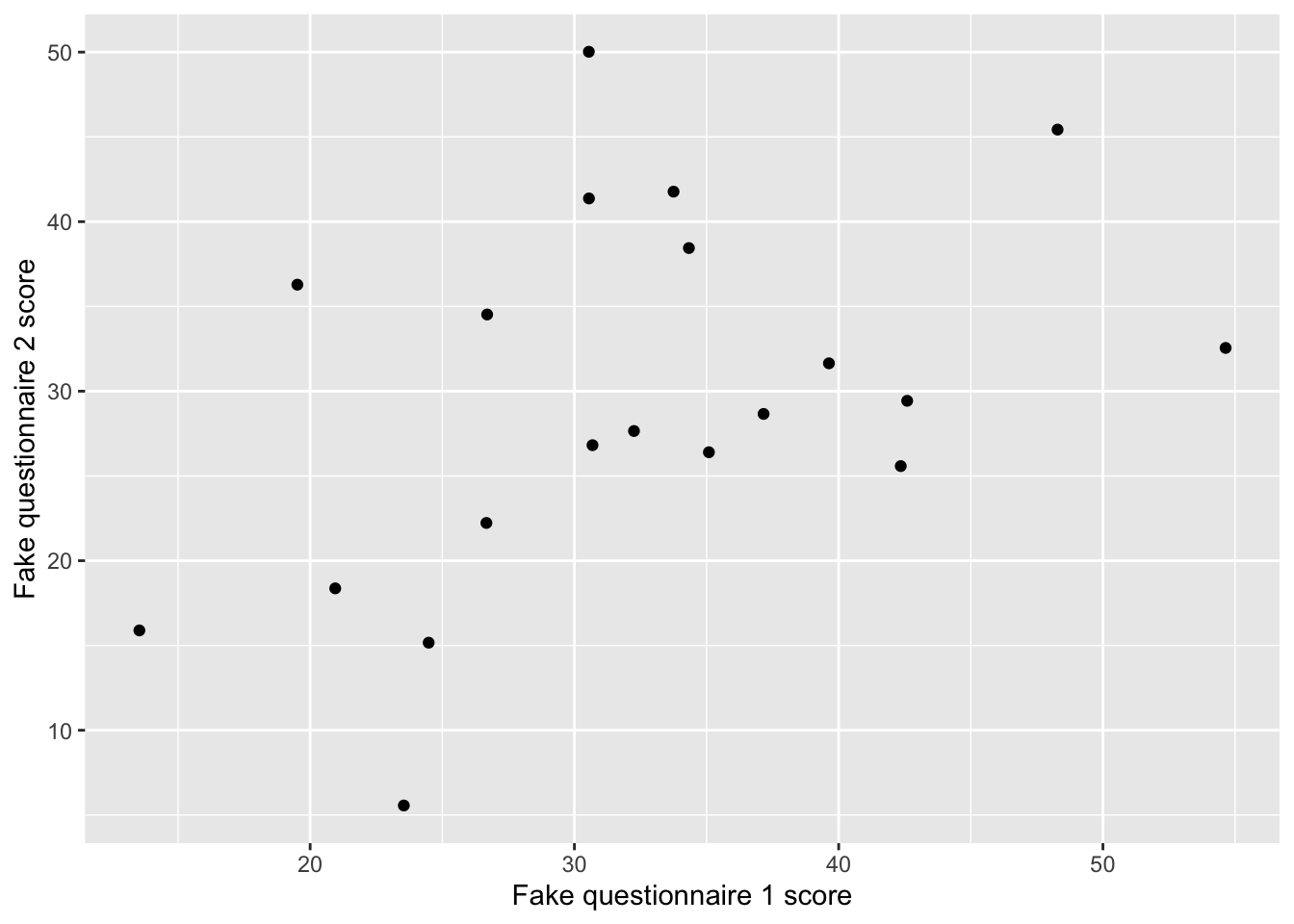

It works! I also think it reads cleanly, because the very first line of the function call tells you which df you’re about to plot. Do be aware, though, that ggplot’s layer-building requires that you chain ggplot calls with +, not %>%. It’ll throw an error if you try, though, so if you mix it up (as I often do) it’s okay.

Now, we can pipe our df through other data manipulation functions before piping it into a ggplot() call, and these changes to the df will only apply to the data being plotted.

What if we want to plot our fake subjects’ d’ values, but with standard error bars using the coefficient standard errors from each individual subject’s model? We can unnest() the coefs column our nested df that contains the individual-subject models and clean the data, just for this plot.

nested_with_models %>%
  # unnest the coefs column to get it into the main df
  # drop other list-columns first just to make the input data smaller
  select(-models, -trials) %>% 
  unnest(coefs) %>%
  # I only want to plot the estimate values for the term is_old, which is the d' term
  filter(term == "is_old") %>%
  ggplot(aes(x = id, y = estimate)) +
  geom_errorbar(aes(ymin = estimate - std.error, ymax = estimate + std.error), width = 0) +
  geom_point() +
  labs(x = "Subject number (arbitrary order)", y = "Fake d' (memory sensitivity)")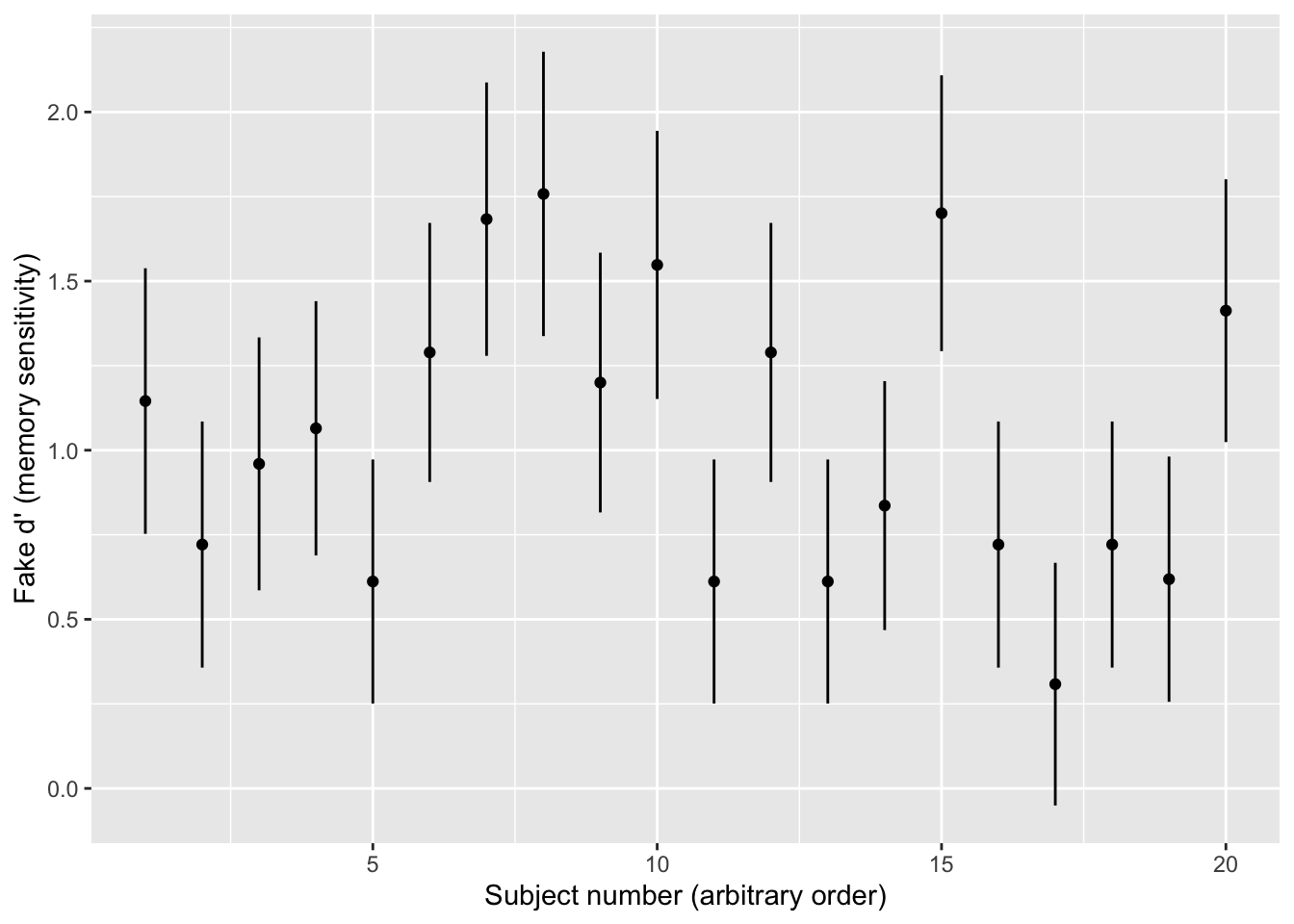

Using this syntax, you can smoothly and legibly pipe your data through pre-processing calls before it gets plotted. You can use this to recode() factor levels so that you get more informative labels in legends, filter() data to plot only certain conditions, or mutate() to create a new helper variable just to plot.