Bayesian Multilevel Modeling with brms
Created by: Paul A. Bloom
extra
R
Links to Files
The files for all tutorials can be downloaded from the Columbia Psychology Scientific Computing GitHub page using these instructions. This particular file is located here: /content/tutorials/r-extra/brms/multilevel-models-with-brms.rmd.
0) Goals for this vignette
- Give a quick intro to multilevel modeling and Bayesian inference
- Show a use case with Brms and some helpful syntax for demonstrating what this model does
- Hopefully, convince you to use multilevel modeling and Bayesian approaches for your stats
1) Why multilevel modeling?
Multilevel modeling, also called ‘hierarchical’, or ‘mixed-effects’ modeling is an extrordinarly powerfull tool when we have data with a nested structure!
A few tutorials on multilevel modeling:
- An awesome visual introduction to multilevel models
- Tristan Mahr’s Partial Pooling Tutorial Using lme4
- Our tutorial on plotting multilevel models in ggplot2
Is multilevel modeling hard? Why is it worth my time?
There are some challenges, but in R, constructing multilevel models follows a very similar syntax to non-nested models! While making modeling decisions can be difficult, actually running multilevel models in R is pretty intuitive!
In situations with nested data, I think multilevel modeling is almost always worth it because * these models are powerful in accounting for variance resulting from nested structures in the data * these models in many situations can help us reduce our uncertainty about population-level effects and robustly account for noisy data * these models in many cases best match our intuitions about the true structure of the data
What are some examples of situations in which multilevel modeling might be helpful?
I always like to think about whether the data are nested when addressing this question. If the data have a nested, or hierarchical structure, then multilevel modeling is probably a good idea.
Some examples of data nesting:
- In a cognitive experiment, subjects each complete many trials of a task. Here trials are nested within subjects
- In a math intervention program, students in different classes each take a test. Here students are nested within classes
- We have county-level data on heart disease rates from 2017. Here we could nest counties within states
Why not just compute participant-level summaries, and do stats on these? Aren’t these summaries more stable AND easier to work with?
- While this can be a good initial approach, we lose information about the data when we compute a summary of any kind
- While participant-level summaries, such as the mean score across 20 trials within a participant (in the first example above), are indeed more stable than individual trials themselves, this approach assumes that all participants are equally variable and thus should all contribute equally to the results
- Especially when some participants have more trials than others, we might want to take into account that some participants’ individual estimates are more reliable than others
- Taking the summary approach can cause us to misinterpret our certainty about effects AND miss real trends in the data.
I’ve heard about partial pooling in multilevel models, what is this? Why would I want to change my estimates of each participant from their TRUE data?
- Partial pooling is a process by which population-level and individual-level effects are estimated at the same time, and each participants’ estimated effect reflects a weighted combination of their own data and the population average. Becuase this structure considers subjects to be drawn from a population distribution, subjects further away from the population average are ‘pooled’ in.
- While changing estimates of each participant from the raw data seems scary, if we consider that data usually contain noise, then this process can be viewed as adjusting noisy estimates on the subject level based on what we know about group level trends. If subjects have very precise data, and lots of it, their estimates will be adjusted less. If subjects have less data or more uncertain data, they will be pooled more.
- Pooling can also help models become much more robust to outliers, and is especially helpful when different participants have different amounts of data. We’ll see a demo of this soon.
2) Multilevel regression model syntax!
Here is the general syntax for modeling in two popular packages, lme4 and brms. In general, this syntax looks very similar to the lm() syntax in R.
In multilevel regression models, we can let different groups (lets say subjects here) have their own intercepts or slopes or both.
Varying Intercepts:
The syntax for letting each subject have their own intercept would be:
outome ~ predictor + (1|subject)
This is basically the same syntax as an OLS regression such as lm(outcome ~ predictor), except we add the second term to let each subject have their own intercept for this given outcome.
Varying Slopes:
The syntax for letting each subject have their own intercept AND slope would be:
outome ~ predictor + (predictor|subject)
This means that when we are estimating the effect of the predictor on the outcome, we also allow each subject to have their own (simultaneously estimated) effect for the predictor on the outcome, as well as the intercept.
3) Setting up the data
We’ll use a simulated dataset for this vignette, so you don’t need to worry about any dependencies involving datasets you don’t have access to while you’re following along. This dataset was created by Monica Thieu initially in the Tidyguide tutorials, so we’ll use a very similar one here. If you have tidyverse loaded, all this code should run if you try to run it in your R console.
Simulate Data
# 20 fake subjects, 50 fake trials per subject

# Will simulate the person-level variables FIRST,
# then expand to simulate the trial-level variables
raw <- tibble(id = 1L:20L,
              age = sample(18L:35L, size = 20, replace = TRUE),
              # assuming binary gender for the purposes of this simulation
              gender = sample(c("male", "female"), size = 20, replace = TRUE)) %>%
  # simulating some "questionnaire" scores; person-level
  mutate(q_1 = rnorm(n = n(), mean = 30, sd = 10),
              q_2 = rnorm(n = n(), mean = 30, sd = 10),
              q_3 = rnorm(n = n(), mean = 30, sd = 10)) %>%
  # slice() subsets rows by position; you can use it to repeat rows by repeating position indices
  slice(rep(1:n(), each = 50)) %>%
  # We'll get to this in a bit--this causes every "group"
  # aka every set of rows with the same value for "id", to behave as an independent df
  group_by(id) %>%
  # I just want to have a column for "trial order", I like those in my task data
  mutate(trial_num = 1:n(),
         # Each subject sees half OLD and half NEW trials in this recognition memory task
         is_old = rep(0L:1L, times = n()/2),
         # I'm shuffling the order of "old" and "new" trials in my fake memory task
         is_old = sample(is_old),
         response = if_else(is_old == 1,
                            rbinom(n = n(), size = 1, prob = runif(1, 0.75, 0.99)),
                            rbinom(n = n(), size = 1, prob = runif(1, 0.11, 0.55))),
         rt = rnorm(n = n(), age/80, sd = .2) + # a real effect of age
           ifelse(is_old ==1, runif(n=n(), .5, 1), runif(n=n(), 0, .5))) %>%
  ungroup()


# Subject 9 is an outlier, and also has fewer trials
raw = mutate(raw,
             rt = ifelse(id == 9, ifelse(is_old ==1, runif(n(), 0, 1), runif(n(), 2, 3)), rt)) %>%
  filter(., !(id == 9 & trial_num > 5))
Raw reaction times for each subject
ggplot(raw, aes(x = factor(is_old), y = rt)) +
  geom_jitter(size = .5, alpha = .5, height = 0, width = .1) +
  facet_wrap('id') +
  stat_summary(fun.data = 'mean_cl_boot', color = 'red', alpha = .5) +
  labs(x = 'Stimulus Seen (1) vs. New (0)', y = 'Response Time (s)', title = 'Raw Data By Subject')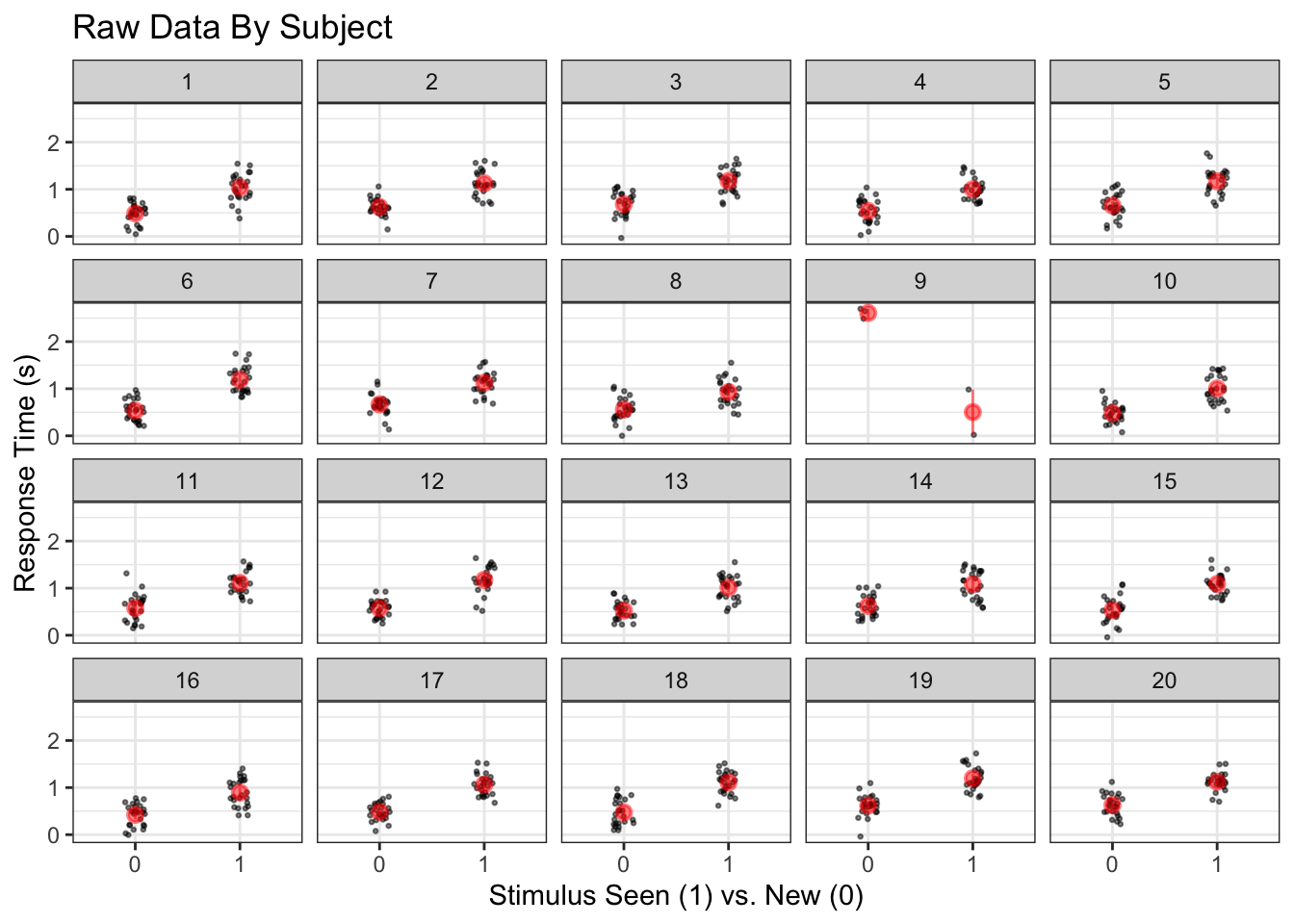
Fancy tidveryse stuff to make a model for each participant.
See Monica’s extreme tidy bible.
Make a linear model for each participant to look at the effect of is_old, or having seen the stimulus before
nested <- raw %>%
  group_by(id, age, gender, q_1, q_2, q_3) %>%
  group_nest(.key = "trials")

nested_with_models <- nested %>%
  mutate(models = map(trials, ~lm(rt ~ is_old, data = .)),
         coefs = map(models, ~tidy(.)))
Plot the estimated effect of is old for each subject
indivModelSummaries = nested_with_models %>%
  dplyr::select(-models, -trials) %>%
  unnest(coefs) %>%
  filter(., term == 'is_old')

ggplot(indivModelSummaries, aes(x = id, y = estimate)) +
  geom_errorbar(aes(ymin = estimate - 2*std.error, ymax = estimate + 2*std.error, width = 0)) +
  geom_point(color = 'purple') +
  labs(x = 'Subject ID', y = 'Estimated Effect of Seen Items on Response Time', title = '1 Model Per Subject') +
  geom_hline(yintercept = 0, color = 'red', lty = 3) +
  ylim(-5, 1)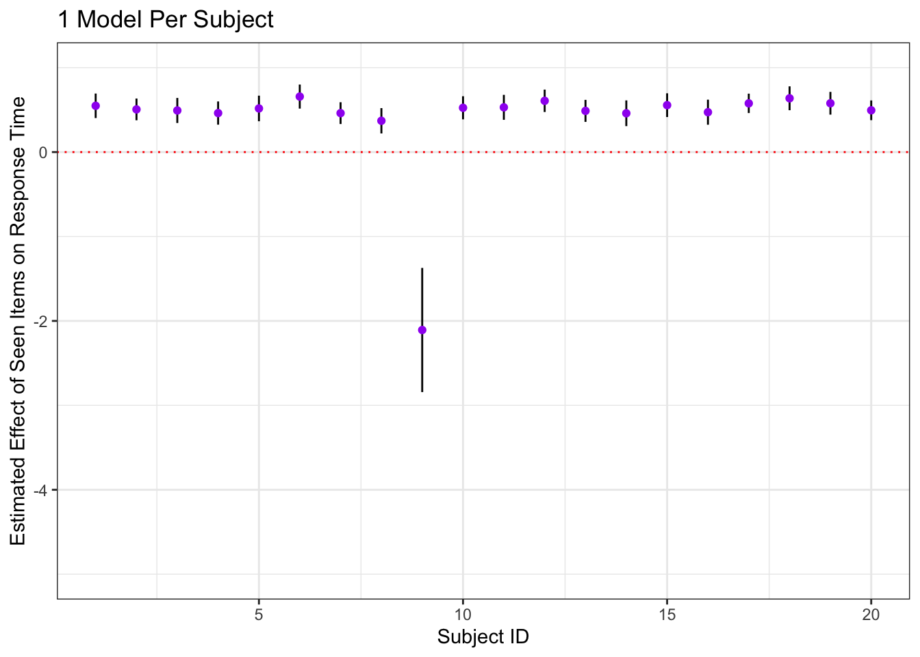
4) Individual Summary (no pooling) and multilevel model comparison!
A model on the summary data with no pooling
rawMeans <- raw %>%
  dplyr::group_by(id, is_old, age) %>%
  summarise(meanRT = mean(rt))
## `summarise()` regrouping output by 'id', 'is_old' (override with `.groups` argument)noPoolModel <- lm(data = rawMeans, meanRT ~ is_old*age)
summary(noPoolModel, digits = 4)Okay, now let’s construct the multilevel model!
multiModel <- brms::brm(data = raw, rt ~ is_old + age + (is_old|id))Compare multilvel model subject-level estimates for the effect of is_old to those from the no-pooling model
a <- summary(multiModel)## Warning: There were 147 divergent transitions after warmup. Increasing
## adapt_delta above 0.8 may help. See http://mc-stan.org/misc/
## warnings.html#divergent-transitions-after-warmupfixedEffect <- a$fixed[2,1]
subjectEffectEstimates <- data.frame(ranef(multiModel)[[1]]) %>%
cbind(indivModelSummaries) %>%
mutate(Estimate.is_old = Estimate.is_old + fixedEffect)
ggplot(subjectEffectEstimates , aes(x = id, y = Estimate.is_old)) +
geom_errorbar(aes(ymin = Estimate.is_old - 2*Est.Error.is_old, ymax = Estimate.is_old + 2*Est.Error.is_old, width = 0)) +
geom_point(color = 'red') +
labs(x = 'Subject ID', y = 'Estimated Effect of Seen Items on Response Time (+/- 2sd)', title = 'Partial Pooling (red) vs. No Pooling (purple)') +
geom_hline(yintercept = 0, color = 'red', lty = 3) +
ylim(-5, 1) +
geom_point(data = indivModelSummaries, aes(x = id, y = estimate), color = 'purple', position = position_nudge(.2)) +
geom_errorbar(data = indivModelSummaries, aes(x = id, y = estimate, ymin = estimate - 2*std.error,
ymax = estimate + 2*std.error, width = 0),
position= position_nudge(.2))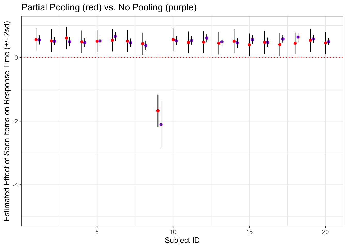
Multilevel model predictions for the age effect
grid <- expand.grid(age = 18:35, is_old = c(1,0))
partialPoolPredicts <- fitted(multiModel, newdata = grid, re_formula = NA) %>%
  cbind(grid, .)


ggplot(partialPoolPredicts) +
  geom_ribbon(aes(x = age, y = Estimate, ymin = Q2.5, ymax = Q97.5, group = is_old), alpha = .3) +
  geom_line(aes(x = age, y = Estimate, group = factor(is_old), color = factor(is_old)), lwd = 2) +
  labs(y = 'Estimated RT', title = 'Multilevel Model Age Effect Estimates\nPoints Are Raw Means') +
  geom_point(data = rawMeans, aes(x = age, y = meanRT, color = factor(is_old))) +
  scale_color_brewer(palette = 'Set1')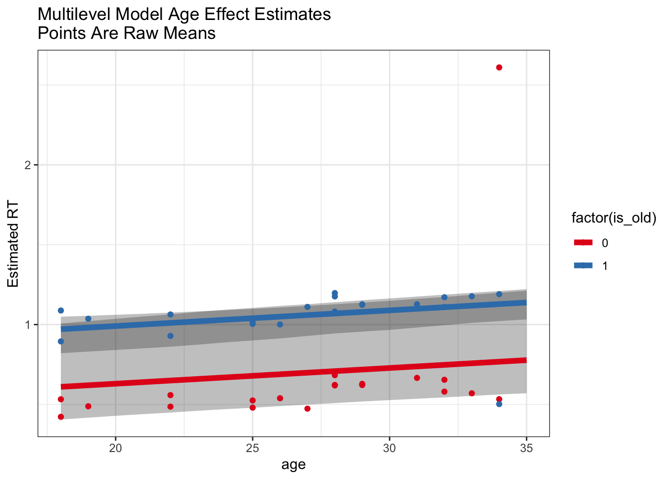
Check out the model predictions from the no pool model
noPoolModel <- rstanarm::stan_glm(data = rawMeans, meanRT ~ is_old*age)noPoolPredictions <- posterior_linpred(noPoolModel, newdata = grid)
noPoolPredictions <- t(cbind(apply(noPoolPredictions,2, quantile, c(.025, .5, .975))))
noPoolPredictions <- cbind(grid, noPoolPredictions)
ggplot(noPoolPredictions) +
geom_ribbon(aes(x = age, ymin = `2.5%`, ymax = `97.5%`, group = factor(is_old)), alpha = .3) +
geom_line(aes(x = age, y = `50%`, color = factor(is_old)), lwd = 2) +
geom_point(data = rawMeans, aes(x = age, y = meanRT, color = factor(is_old))) +
labs(y = 'Estimated RT', title = 'Two-Stage Model Estimates (no pooling)\nPoints Are Raw Means') +
scale_color_brewer(palette = 'Set1')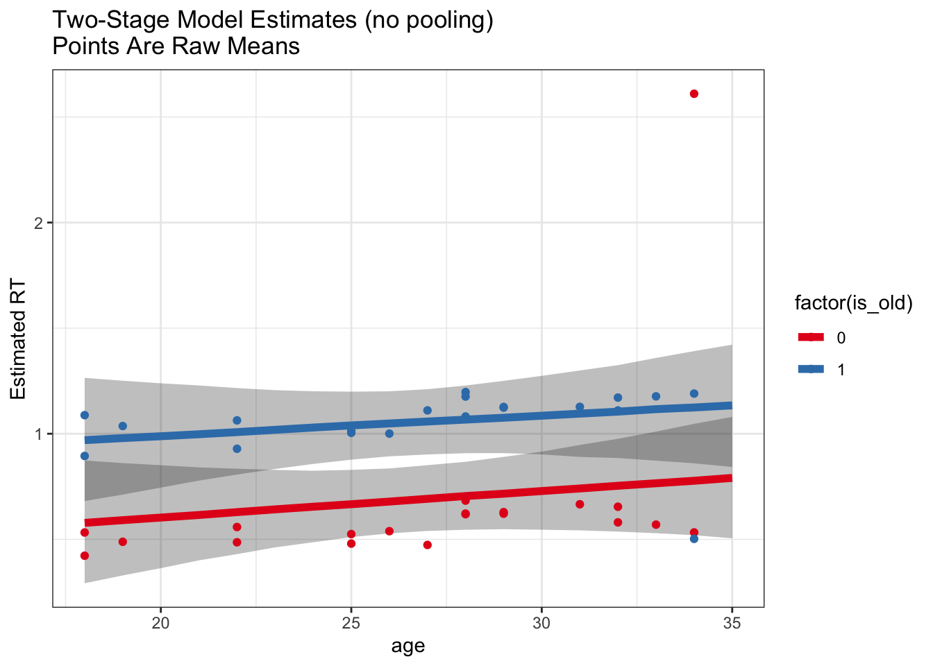
So, we can see from this example that the use of the multilevel model helps us recover this true effect of age whereas a model based on subject-level summaries is not as robust to outliers.
Is this just because of outliers?
This is a particularly clean example where we KNOW that one subject is an outlier who was not doing the experiment the same way. Usually we don’t have that luxury, so multilevel modeling gives us a big advantage in being able to include all the data and allowing the model to estimate effects in a manner robust to potential outliers.
This is more of a philosophical point, but in general it can be very hard (and sometimes a confound) to decide when to exclude subjects or trials. We can define cutoffs, but we may still get outliers within these cutoffs. Even with reasonable outlier exclusion rates, we often see that multilevel models help to model the data in a manner more robust to outliers.
5) What about the Bayesian stuff?
The Bayesian aspect of multilevel modeling was implicit in much of this tutorial today, but we didn’t really focus on it. However, Bayesian software like brms lends itself particuarly well to multilevel modeling frameworks where there are many parameters and optimization is complex – bayesian approaches will still give us models that don’t fit well if the data are too sparse (and we don’t set regularizing priors) but they won’t fail to converge in the same way maximum likelihood models do.
We haven’t talked much about the difference in approach when using Bayesian as opposed to frequentist modeling today – more on that soon!